


















Article ID: CM2601102004
Views: 21Explainable Forecasting of Anomalous Operational States Using Multivariate Cloud Telemetry
 PDF
PDF
⬇ Downloads: 0
1. INTRODUCTION
Cloud-based IT services are a cornerstone of today’s digital infrastructure. They can run mission-critical applications in the financial, healthcare, e-commerce, media streaming, and enterprise IT sectors [1, 2]. Cloud elasticity is becoming a cornerstone of cloud computing, helping organisations become scalable, available, and cost-effective [3]. This dependency also increases the risk of disruption; if service is interrupted for any reason, it can result in financial losses, service level agreement (SLA) breaches, reputational damage, and a loss of user trust [4, 5]. As cloud systems grow in size, scope, and complexity, service availability is increasingly a critical operational reliability concern.
Outages are unlikely to be caused by one single failure point in a cloud environment. They tend to result from pervasive resource pressure, compute workload bursts, and poor interactions among compute, memory, storage, and network elements [6]. However, many operational monitoring systems still use hard-coded threshold alerts that trigger only when a metric crosses a threshold [7]. This reactive approach often fails because it is too late to prevent failure. Fixed thresholds also struggle to adapt to dynamic workloads and heterogeneous service behaviour, resulting in too many false alerts and too few alerts for critical events. These constraints drive the need for smarter, more predictive methods of cloud reliability management.
This study takes a different perspective on service outages, defining outage risk as a time-varying process rather than a series of one-off, discrete events. Unusual cloud activity can manifest as slow changes in telemetry data, such as CPU saturation, increasing memory pressure, network performance fluctuations, or growing disk activity [8]. These indicators can happen before the service is interrupted and can thus be modelled as potential service outage indicators. For this reason, outage-risk management is considered a forecasting problem in this context, not just a task to be done after an incident.
Early-warning systems that predict outage risk have benefits over traditional fault-detection systems. Operators can use predictive analysis to anticipate and address cumulative stress and progressive degradation before users notice, which could limit downtime and operational impact [9]. This view aligns with trends in AIOps and site reliability engineering towards data-driven decisions that support incident response, rather than a reactive approach [10]. But this is not possible without models that are reliable and learn temporal dependencies in high-dimensional operational data in a reliable and interpretable way.
Many papers have focused on anomaly detection and failure diagnosis in cloud systems, but there are several limitations. First, most investigations rely on a single evaluation metric, such as CPU utilisation or memory utilisation, rather than characterising relationships across resource dimensions [11]. This is not an accurate representation, because outages often occur when multiple metrics are stressed, not just when one spikes. Second, most of the literature focuses on post-incident anomaly detection; that is, it detects abnormal behaviour only after service degradation has occurred. These can be diagnostically valuable, but offer little warning for prevention. Third, anomaly detection does not necessarily equal outage forecasting; detecting an anomaly does not mean a service disruption.
Many black-box machine learning and deep learning models also lack transparency. In operational environments, trustworthy predictions and actions are hard to achieve, particularly when alerts can trigger automatic or semi-automatic mitigation [12]. If models are not explainable, reliability engineers may be less likely to adopt them, and even when they are correct, they may be less useful. These issues highlight the need for multivariate, explainable outage-risk predictive frameworks.
Cloud monitoring and AIOps knowledge has been maturing, but a gap remains. Very few publicly available frameworks still support explainable forecasting of IT service outage risk. Numerous studies use operational data that are unavailable, which limits comparisons between studies. Further, cloud telemetry is often underused, and lagged effects, rolling trends, and escalation patterns that lead to degradation are generally poorly reported. The field also needs to address rare-event prediction under class imbalance and control false alerts. The fusion of these capabilities, such as forecasting, cross-resource telemetry fusion, temporal learning, and explainability, is therefore not thoroughly explored.
This study aims to address these gaps by achieving three objectives. First, it builds a predictive analytics model to estimate future abnormal service operation states based on cloud telemetry data, using abnormal cloud service indicators only as surrogate measures of possible service degradation. Second, it incorporates CPU, memory, disk I/O, network I/O, lagged values, rolling statistics, and slopes; it also includes relationships between resources not derived from labels, while excluding workload type from the principal predictor set to minimise proxy leakage. Third, SHAP values provide interpretable predictions so that reliability engineers can investigate the factors driving a prediction. The novelty is not algorithmic but methodological integration: several well-known methods of modelling, evaluation, and explainability are integrated, and the model’s strength and robustness are assessed while accounting for data imbalance. The contribution introduces a leakage-controlled forecasting workflow that combines multivariate telemetry processing, temporal feature engineering, imbalance-aware assessment, robustness validation, and operational interpretation.
This contribution is presented as an application of an AIOps framework rather than a new learning algorithm. These techniques – lagged features, rolling statistics, LSTM forecasting, and SHAP explanations – are well-known. Still, the innovation is combining them into a leakage-controlled, multivariate anomaly-risk forecasting pipeline that leverages an open dataset, imbalance-aware evaluation, false-alert analysis, episode-onset warning-coverage analysis at a preselected forecast window, and explainability. The study is not only anomaly-tagged, but it also forecasts these operational states instead of just detecting them as anomalies; it evaluates 31 different predictors derived from the telemetry signal data, but under class imbalance, it compares linear, bagged-tree, gradient-boosting, and sequence models, and interprets the resulting risk scores using SHAP. Workload type is not included in the main set of predictive features because it is highly correlated with the dataset label; it is included in the diagnostic and sensitivity analysis.
The operational interpretation is intentionally limited to early anomaly warning. We use an exact three-step-ahead target, and the data sampling interval has a median of 60 seconds, resulting in a nominal three-minute forecast horizon. The latency of mean model-only inference was less than 0.001ms per sample for the Logistic Regression model, and around 0.028ms, 0.003 ms, and 0.037ms per sample for Random Forest, XGBoost, and LSTM, respectively. These values are based on model inference only; a pipeline with live data would also require telemetry ingestion, processing, communication, orchestration, and possible human approval. Therefore, the three-minute anomaly forecast should not be treated as a three-minute warning before a customer-visible outage.
2. LITERATURE REVIEW
2.1. IT Service Reliability and Outage Analysis
In large-scale distributed and cloud systems, researchers have extensively studied IT service reliability and availability, as the coordinated behaviour of heterogeneous infrastructure components affects cloud service availability [13]. Previous studies list resource exhaustion, workload peaks, cascading failures, configuration errors, and software bugs as some of the most common causes of cloud-service outages. Cloud environments differ from monolithic systems because interdependencies among compute, storage, and networking layers can cause localised stresses to cascade rapidly into service-level degradations [14]. Hence, outages often result from accumulated operational pressures rather than a single failure.
Traditional site reliability engineering (SRE) processes monitor key performance indicators (KPIs), establish service-level objectives (SLOs) [15], and react to static or dynamic alerts. These practices improve observability and incident response but remain largely reactive. Monitoring techniques typically detect abnormal behaviour only after a set threshold is exceeded, so they fail to anticipate the onset of degradation. Furthermore, when a cloud-based system contains elastic and variable workloads, thresholds may be difficult to model because normal operating ranges change across services and time periods [8, 16]. Thus, traditional reliability monitoring is not very effective at predicting failure before it becomes operationally relevant.
2.2. Anomaly Detection in Cloud and Distributed Systems
Previous studies around cloud failure management have mainly focused on anomaly detection. Common statistical tools include z-score analysis, moving averages, and control charts, which are simple and easy to understand [17]. These methods are generally stationary or distributionally regular; however, this assumption does not hold for cloud telemetry. To overcome these limitations, researchers have proposed machine learning techniques such as clustering, isolation forests, autoencoders, and probabilistic graphical models to find nonlinear patterns in high-dimensional monitoring data.
In many cases, machine learning substantially improves anomaly-detection accuracy, but most existing approaches are, by nature, retrospective [18]. They detect abnormal behaviour only after it occurs, so they offer limited value in proactively preventing outages [19]. Another limitation is that these models may be confused by benign workload variation, leading to more false positives [20]. Importantly, an anomaly isn’t necessarily an outage precursor, as some anomalies are short-lived and self-resolving. These limitations show the need to complement detection models with prediction models to estimate the likelihood of service failure.
2.3. Predictive Analytics and AIOps
AIOps is a paradigm change from reactive monitoring to predictive and automated IT operations. It is similar to predictive maintenance in industrial systems, using sensor data to predict equipment failure before it occurs. The same principle holds in cloud environments: If cloud resource usage is treated as a temporal forecasting problem, the data can be used to detect early indicators of service degradation.
While the concepts align, predictive modelling in IT operations faces several technical challenges. Outage events are extremely rare, leading to class imbalance that may bias standard learning algorithms [21]. Operational data are also noisy due to workload variability, deployment activity, and measurement artefacts. Cloud environments are not stationary, and new configurations and workload profiles can cause temporal drift [22]. Deep learning models like recurrent neural networks and temporal convolutional networks can learn sequential dependencies [23], but they lack interpretability and operational trust in AIOps. Predictive analytics thus supplements, rather than replaces, existing reliability practices.
2.4. Multivariate Operational Telemetry
One shortcoming often noted in previous studies is the focus on a single resource or narrowly defined telemetry sources. Studies analysing CPU, memory, or network usage alone may not capture the interdependencies among cloud resources that drive complex degradation patterns. When workloads generate compounded resource contention, several resources are likely to be affected by service degradation: CPU, memory, disk I/O, and network [24]. These interactions can make predictions difficult and limit the ability to generalise for different workload types.
Metrics for compute, memory, storage, and networking resources have attracted interest in a growing number of recent studies on cross-resource telemetry fusion [5]. These methods provide a more holistic view of system health by accounting for cross-resource relationships and temporal dynamics. However, many current studies still focus on anomaly detection or root-cause analysis without considering future outage-risk forecasting. Multi-source models may be more complicated, complicating feature selection, model understanding, and computation. These trade-offs encourage a feature-engineering strategy that balances predictive power with operational ease.
2.5. Explainable AI for IT Operations
A critical need for using machine learning in IT operations is explainability. Reliability engineers need to know not only what a model predicts, but also why it predicts that. If the predictive model’s outputs feed into mitigation decisions, the model’s behaviour becomes opaque, and operators may lose trust in it and be unable to judge whether an alert reflects credible operational risk [12]. Explainable AI has thus emerged as a crucial demand in AIOps research and practice.
Other approaches like SHAP and LIME can explain the contribution of individual features to predictive risk and link these explanations to operational metrics such as disk contention, memory pressure, and CPU saturation, enhancing actionability [25]. However, previous research usually applies explainability at the end of static modelling [26, 27]. This limits the immediate usefulness of XAI in real-world IT service management.
2.6. Summary and Identified Gap
In conclusion, although significant progress has been made in cloud monitoring, anomaly detection, and cloud diagnostic analysis, gaps remain in forecasting regarding explainability and reproducibility. Much of the literature uses detection-oriented methods that offer little warning, and class imbalance, temporal drift, and limited interpretability remain problematic for predictive analytics. Cross-resource telemetry fusion has become a key factor; however, many studies focus on future-risk forecasting without providing operational interpretations.
Proprietary datasets also limit reproducibility and comparative analysis. Hence, evaluation of explainable, multivariate outage-risk prediction based on publicly accessible heterogeneous operational data remains underdeveloped. To address this, this work introduces an integrated framework that integrates temporal predictive modelling, multivariate feature engineering, imbalance-aware evaluation, and explainable decision support. It therefore contributes in practice and methodology, not by offering novelty in any individual element such as lag features, rolling statistics, LSTM, or SHAP.
2.7. Novelty Positioning Against Existing Literature
The study’s novelty lies in the integrated forecasting workflow rather than in any individual algorithmic component. The workflow combines multivariate telemetry, temporal feature engineering, class-imbalance handling, validation-based model selection, episode-onset warning-coverage analysis at a prespecified horizon, false-alert evaluation, robustness testing, and SHAP explanations in a single anomaly-risk forecasting study. This positioning avoids overstating algorithmic novelty while clarifying the practical methodological contribution.
3. METHODOLOGY
3.1. Dataset Description
This research used the open Cloud Resource Usage Dataset for Anomaly Detection. The final implementation included 14,400 observations, 10 user streams, and 1,440 unique timestamps from 2025-07-01 00:00:00 to 23:59:00, with a median sampling interval of 60 seconds. Each observation includes CPU usage, memory usage, disk I/O, network I/O, workload type, user identifier, and an anomaly label. In the public dataset description, anomaly labels are defined as signals of resource overuse, including hidden anomalies, but without a precise, deterministic formula for generating labels. Thus, this manuscript does not infer the provenance of the label beyond the published description. Empirically, 1,257 labels were observed in Crypto Mining, and all of them were positive, which accounts for 85.7435% of all the observed labels, and the rule Crypto Mining with CPU usage at least 80% matched 99.9931% of the observed labels with one mismatched label. Workload type was therefore an unusually strong proxy for the label and was omitted from the main set of predictive features and examined individually in a sensitivity analysis.
The data set does not include records of confirmed production outages, but it could be used to control an environment to determine whether temporal telemetry patterns can be predicted for abnormal operational states. The goal of this research is not to directly predict outages visible to the customer, but to assess the potential of an explainable early-warning system that uses a middle layer of abnormal system behaviour as a warning signal.
We mathematically represented the dataset as a multivariate time series.

The vector of observations at time t is called x_t, and the corresponding label of anomaly at time t is called y_t. The original analysed variables have no missing values during the observation period, so no pre-observation period and no imputation are needed before feature engineering. While there are 14400 rows, these are divided across 10 parallel user streams, each covering only 1440 different one minute timestamps, which has implications as noted in the Limitations section below.
3.2. Outage Proxy Definition
Availability reports for confirmed IT service outages are hard to come by since outages are often a matter of confidentiality and related to in-house operations. An anomaly label is used as a proxy for this, so that the study includes only the potential causes of a service disruption rather than service disruption itself. This is important to note, because the model is predicting the probability of anomaly events that are precursors to a production outage, and not the actual production outage. This is in line with the AIOps literature that indicates that abnormal telemetry can last for a long time before service degradation or service unavailability occurs.
The principal modelling target was the exact anomaly label three observations ahead rather than a rolling-OR or sustained-anomaly proxy. For user stream  and anchor time
  , let
, let  denote the 31-feature engineered predictor vector and
  denote the observed anomaly label. The primary forecasting target was
  implemented by shifting the anomaly label by three observations within each user stream. Each classical model therefore used to predict
  For the LSTM, the 12-step input sequence consisted of
  and this complete sequence was paired with the same target The
  target alignment was completed before model-ready observations were counted and before LSTM sequence generation; therefore, the three-step horizon was not subtracted again when calculating the 987 development sequences or 417 held-out sequences per user.
A secondary sustained-anomaly sensitivity analysis was conducted to examine whether conclusions changed when a positive state required at least k consecutive anomaly labels. For k = 2, the held-out set contained 42 positive observations (1.0072%) forming 21 episodes. For k = 3 and k = 5, no positive held-out observations or episodes remained; therefore, precision, recall, F1, PR-AUC, false-alert rate, and warning coverage were not estimable for those settings. The sustained definitions were treated as sensitivity analyses only and did not replace the exact primary target.
3.3. Exploratory Data Analysis
The statistical characteristics, variation, and correlations of cloud resource metrics were explored first through exploratory data analysis before the model was built. It was not an inferential objective, but rather a diagnostic objective: the analysis was used to understand the distributional skewness, variance, and extreme values to guide in feature engineering and model selection. Cloud telemetry data exhibit this kind of skewness and variance because workloads are inherently bursty and elastic.
Workload heterogeneity was also taken into account, due to different types of services generating different resource-utilisation patterns. For instance, a workload that uses a lot of CPU computations can cause the CPU to become overloaded, while a data-driven workload might require more memory and disk I/O. Inter-dimensional relationship of resources was explored to find correlation in the behaviour which could signify cascaded stress. The results of these observations warranted use of multivariate features and cross-resource dependencies in the predictive model.
3.4. Data Preprocessing
Before feature extraction and model training, telemetry validity checks were applied. The implementation identified 23 CPU values below 0%, one CPU value above 100%, and 285 negative Disk I/O values. CPU usage was clipped to the physically valid 0–100% range and negative Disk I/O values were clipped to zero before feature engineering and standardisation. After cleaning, CPU ranged from 0 to 100 and Disk I/O from 0 to 69.70. Continuous predictors were then standardised using means and standard deviations estimated exclusively from the training partition, with the same training-derived parameters applied to held-out data to prevent leakage.

where  denotes the observed value of feature
  at time , while
  and
and  denote the mean and standard deviation of feature
  , respectively, calculated exclusively from the training partition. The same training-derived parameters were subsequently applied to the validation and test partitions to prevent information leakage.
Temporal splitting was performed chronologically and separately within each of the 10 user streams after feature engineering and exact t+3 target alignment. Each original user stream contained 1,440 observations; the 12-observation rolling feature calculations made the first 11 positions unavailable, while the t+3 target shift made the final three positions unavailable, leaving 1,426 model-ready anchor–target observations per stream. The first 998 model-ready observations formed the development partition and the final 428 observations formed the held-out test partition. For classical-model hyperparameter selection, the first 898 development observations were used for fitting and the final 100 observations were used for chronological validation. For the LSTM, 12-step sequences were first generated across the complete 998-observation development partition, producing 998 − 12 + 1 = 987 development sequences per user; these were then split chronologically into the first 888 fitting sequences and the final 99 validation sequences. Within the held-out partition, 428 − 12 + 1 = 417 complete test sequences were available per user, producing 4,170 common aligned held-out sequences across the 10 user streams. No LSTM sequence crossed a user-stream or development/test boundary; because the LSTM fitting/validation split was applied after development-sequence construction, adjacent fitting and validation sequences could share historical input observations. Although validation targets occurred strictly after fitting targets, shared historical inputs near the fitting/validation boundary may introduce limited dependence between the two subsets; future work should evaluate a purged temporal validation gap that removes all shared input history.
3.5. Feature Engineering
The purpose of feature engineering was to include both the current state of the system and its history. Lagged features were created from past observations of these continuous resource metrics (CPU usage, memory usage, disk I/O, and network I/O) in each user stream, which allowed the models to feed in the latest historical resource behaviour.

Rolling statistical features were derived from sliding windows, for example, rolling means and rolling variances, and slope features were derived to identify short-term trends in the resources.

CPU_Burst was calculated via the implemented first difference rule to detect a sudden CPU increase, and CPU_Memory_Corr was computed as the 12-observation rolling Pearson correlation of CPU and memory use. These features are able to capture short time periods of CPU spikes and cross-resource dependence without any workload type and label information. These designed attributes combined transformed raw telemetry into a representation that was appropriate for predictive learning. The rolling means, variances, and CPU–memory correlation were calculated using a 12-observation rolling window, as was the implementation parameter ROLLING_WINDOW = 12. The 12 observation rolling window summarised around 12 minutes of the past telemetry.
3.6. Predictive Models
Four predictive models were compared using a shared chronological hold-out design. Logistic Regression was used to get the linear baseline. Non-linear tree-based interactions were modelled by Random Forest. XGBoost is also added as a more robust baseline gradient boosting model that can take advantage of engineered features such as lag, rolling, slope, burst, and cross-resource features without any memory of the sequences. The LSTM received 12-step sequences and modelled temporal dependencies directly through gated recurrent states. Including XGBoost and engineered temporal predictors creates a stronger comparison than evaluating the LSTM only against static linear and bagged-tree baselines. The amount of historical information was not identical across model classes. Each classical model received a single 31-feature vector at anchor time t, whose longest engineered rolling features used raw telemetry from t – 11 through t, corresponding to an effective history of up to 12 observations. The LSTM received 12 consecutive engineered vectors from t – 11 through t; because the earliest vector in that sequence itself contained a 12-observation rolling summary, the LSTM could indirectly access raw telemetry as far back as t-22, corresponding to an effective history of up to 23 observations. The comparison should therefore be interpreted as a comparison of complete forecasting pipelines rather than as a controlled architecture-only comparison under matched temporal receptive fields.


where x_t is the engineered feature vector constructed from the telemetry observations up to time t, β_0 is the intercept, β is the vector of the model coefficients, and p ̂(t+h) is the estimate of the probability of an anomalous operational state at time t+h. Logistic Regression offers a simple yet interpretable baseline model that is computationally efficient, but has the limitation of a linear decision function which does not support more complex interactions and sequential escalation processes.
To capture the interactions of nonlinear features, an ensemble of decision trees, the Random Forest Classifier, was used. The model does not include nonlinear interactions, but each engineered instance is modelled separately, which is not as flexible as direct modelling of sequential interactions. Therefore, a long short-term memory (LSTM) network was chosen to model explicitly the temporal dynamics. The LSTM can hold the information from previous time steps by using gated memory mechanisms, which can learn the escalation trajectories that could be precursors to outages.
In addition to the four principal predictive models, static CPU/memory threshold alerting and a user-specific EWMA CPU score were implemented as exploratory operational reference baselines on the same common aligned held-out set. The static reference generated a positive score when CPU usage exceeded 75% or memory usage exceeded 75%. The EWMA reference used a 12-observation CPU EWMA with adjust=False, calculated the CPU residual relative to the EWMA, scaled the residual by its population standard deviation, and transformed it to a 0–1 score using the logistic function. These operational references were retained separately from the four-model architectural comparison.
3.7. Implementation Details
Experiments were conducted in Python using NumPy and Pandas for preprocessing, scikit-learn for Logistic Regression and Random Forest, XGBoost for gradient boosting, PyTorch for the LSTM, and SHAP for explanation. Classical-model hyperparameters were selected from 11 prespecified candidate configurations using chronological validation PR-AUC as the sole selection criterion. Logistic Regression evaluated C ∈ {0.1, 1.0, 10.0}, and C = 0.1 was selected with validation PR-AUC=0.089369. Random Forest evaluated four configurations: 200 trees with depth 6 and minimum leaf size 2; 200 trees with depth 10 and minimum leaf size 2; 300 trees with depth 6 and minimum leaf size 4; and 300 trees with depth 10 and minimum leaf size 4. For all Random Forest candidates, min_samples_ split = 2, max_features = sqrt, and class_weight = balanced were fixed. The selected Random Forest used 300 trees, maximum depth 6, and minimum leaf size 4, achieving validation PR-AUC = 0.091260.
XGBoost evaluated four prespecified configurations: 200 estimators with depth 3 and learning rate 0.03; 200 estimators with depth 5 and learning rate 0.05; 400 estimators with depth 3 and learning rate 0.03; and 400 estimators with depth 5 and learning rate 0.05. Subsample=0.90, colsample_bytree = 0.90, min_child_weight = 2, reg_alpha = 0, and reg_lambda = 1 were fixed across candidates. The selected configuration used 200 estimators, maximum depth 3, and learning rate 0.03, with validation PR-AUC=0.078695. The XGBoost positive-class weight was 10.031941 during validation search and 10.138393 after refitting on the complete development partition.
The LSTM architecture was prespecified rather than selected through a separate hyperparameter search. It contained one LSTM layer with 64 hidden units and dropout=0.20, and was trained using Adam with learning rate=0.001, training batch size=64, a maximum of 50 epochs, and early-stopping patience of five epochs. Training batches were not shuffled, validation used batch size 256, and early stopping monitored weighted binary cross-entropy validation loss with a minimum required improvement of  . The positive-class weight was 10.044776, calculated from 8,076 negative and 804 positive LSTM fitting sequences. The final training run stopped after six epochs and retained the checkpoint with the lowest validation loss of 1.214379.
Experiments were executed in a Google Colab Python 3 runtime using CPU execution only; the recorded implementation reported ‘Device: cpu’, and random seeds were fixed at 42 for NumPy, Python’s random module, and PyTorch. Exact transient Colab package-version and hardware-instance metadata were not preserved in the saved run; consequently, the reported computational environment documents the execution platform, device class, libraries, and randomisation controls without claiming exact software-build reproducibility. The workflow loaded and validated telemetry; corrected physically implausible values; constructed 31 telemetry-derived predictors; generated the exact t+3 target within each user stream; performed user-specific chronological fitting, validation, and held-out splitting; generated 12-step LSTM sequences without crossing user or development/test boundaries; fitted the four predictive models; evaluated all models at a fixed 0.50 classification threshold on the common 4,170-sequence held-out set; and conducted feature ablation, workload-inclusion sensitivity, Gaussian-noise robustness, workload-specific evaluation, temporal robustness, sustained-anomaly sensitivity, paired-bootstrap testing, SHAP analysis, episode-onset warning-coverage analysis at the prespecified horizon, prediction-stability analysis, and inference-latency benchmarking.
3.8. Robustness and Statistical Validation Protocol
To strengthen internal reliability, Gaussian-noise, workload-specific, temporal, workload-inclusion, sustained-anomaly, and paired-bootstrap analyses were applied using held-out data. The principal models were not retrained during Gaussian-noise, workload-specific, or temporal robustness evaluation. For Gaussian noise, perturbations were applied to the four cleaned raw telemetry variables in the held-out period and the lag, rolling, slope, burst, and correlation features were recomputed before scoring. Paired bootstrap testing used 1,000 identical resamples across models for F1 and PR-AUC comparisons. Table 1 summarises the purpose, procedure, and reported outputs of the robustness and statistical validation analyses used to assess the reliability of the predictive models.
Table 1. Robustness and statistical validation protocol.
| Test | Purpose | Procedure | Reported Output |
| Gaussian noise stress test | Assess stability under measurement noise | Add zero-mean Gaussian noise equal to 10% of the training-set standard deviation to raw held-out CPU, memory, disk I/O, and network I/O; reapply physical bounds; recompute all engineered features; score without retraining. | Precision, recall, F1, PR-AUC, false-alert rate, ΔF1, ΔPR-AUC |
| Workload-specific robustness test | Assess variation across workload categories | Partition the common aligned held-out set by workload type. Workload type is used only for subgroup evaluation and is excluded from the principal predictor set. | N, positive cases, precision, recall, F1, PR-AUC, false-alert rate |
| Temporal robustness test | Assess short-horizon stability across time | Split the 4,170 aligned held-out forecasting sequences into non-overlapping early (2,080) and late (2,090) segments and score the same fitted models at the same threshold. | Positive rate, precision, recall, F1, PR-AUC, false-alert rate |
| Paired bootstrap significance test | Assess whether model differences exceed sampling variation | Use 1,000 paired bootstrap resamples of identical held-out indices for LSTM versus Logistic Regression, Random Forest, and XGBoost. | Observed difference, 95% CI, two-sided p-value, significance |
The measurement noise, logging delays, and the slight variation of telemetry that occurs in real cloud monitoring systems were taken into account by including the Gaussian noise test. The workload-specific test was added to ensure that the forecasting model was not effective for only one workload type. The temporal robustness test has been added as workloads on clouds may vary over time and a practical outage prediction model should be stable across the various parts of the monitoring horizon. In combination, these tests offer controlled evidence of the robustness of the models, yet recognise that further external generalisation to production scale is required.
3.9. Statistical Significance Testing
A paired bootstrap significance test with 1,000 iterations was carried out to determine if the differences in performances between the LSTM model and the baseline models were statistically significant. Given the imbalanced nature of the outage forecasting task, F1 and PR-AUC were used as the statistics, as they are more suitable metrics for the task. All test instances were held out chronologically in the same manner and ground-truth labels were the same across all models. The pair bootstrap results are used here as an approximate within-sample uncertainty estimate, not as evidence from independent observations in time, since adjacent forecasting windows are not completely independent.
For each bootstrap iteration, test-set prediction windows were sampled with replacement. The same bootstrap sample was applied to the LSTM, Random Forest, XGBoost, and Logistic Regression predictions. For each model, the selected performance statistic was calculated as:

where  represents either the F1 or PR-AUC of model
  during bootstrap iteration
  . The performance difference between the LSTM and each baseline model was then computed as:

The 95% confidence interval was obtained from the 2.5th and 97.5th percentiles of the bootstrap distribution of  . Statistical significance was calculated using a two-sided empirical bootstrap test:

A difference was considered statistically significant when the 95% confidence interval did not include zero and the two-sided bootstrap p-value was below 0.05. This procedure ensured that significance was computed from paired model-performance differences on identical test samples, rather than from an unpaired comparison.
3.10. Evaluation Metrics
Since anomaly events are imbalanced, precision, recall and F1 were prioritised in the performance evaluation:

PR-AUC was used to evaluate ranking performance across decision thresholds under class imbalance, while precision, recall, F1, and false-alert rate were calculated at the prespecified 0.50 classification threshold. The threshold was fixed before held-out evaluation and was not optimised using test labels. The 0.50 threshold was retained as a prespecified common operating point to ensure direct comparability across models and to avoid post-hoc threshold optimisation on the held-out test set; threshold optimisation for deployment-specific precision–recall trade-offs was outside the scope of this proof-of-concept evaluation. Operational suitability was additionally examined through episode-onset warning coverage at the prespecified forecast horizon, prediction stability, and inference latency.
Table 2(a) summarises the training configuration used to maintain temporal realism and controlled optimisation. The window size captures short-term escalation trends, while the forecast horizon reflects a practical early-warning requirement. Chronological splitting reduces leakage risk, and early stopping helps control overfitting. Table 2(b) shows that the final 31-feature predictor set integrates current-state telemetry with lagged, rolling, slope, burst, and cross-resource variables while excluding workload type and all label-derived information.
Table 2(a). Model training configuration.
| Parameter | Value |
| LSTM sequence length | 12 engineered time steps |
| Forecast target | Exact anomaly label at t+3 |
| Nominal horizon | 3 minutes (median sampling interval 60 s) |
| Development/Test split | 70% / 30% chronological within each user stream |
| Validation split | Classical models: first 898 of 998 development observations for fitting and final 100 for validation; LSTM: 987 sequences generated from all 998 development observations, then first 888 sequences for fitting and final 99 for validation. |
| Aligned held-out test set | 4,170 sequences; 341 positives (8.1775%) |
| Predictor count | 31 telemetry-derived features; workload and label-derived variables excluded |
| Decision threshold | 0.50 fixed before held-out evaluation |
| Logistic Regression | C=0.1; lbfgs; L2; class_weight=balanced; max_iter=2000 |
| Random Forest | 300 trees; max_depth=6; min_samples_split=2; min_samples_leaf=4; max_features=sqrt; class_weight=balanced |
| XGBoost | 200 estimators; learning_rate=0.03; max_depth=3; subsample=0.90; colsample_bytree=0.90; min_child_weight=2; reg_alpha=0; reg_lambda=1; scale_pos_weight=10.138393 |
| LSTM | 1 LSTM layer; 64 hidden units; dropout=0.20; Adam learning rate=0.001; training batch size=64; maximum 50 epochs; validation weighted BCE monitored for early stopping; minimum improvement=1×10⁻⁴; patience=5; final run stopped after 6 epochs. |
| Weighted BCE positive weight | 10.044776, calculated from 8,076 negative and 804 positive LSTM fitting sequences. |
| Random seed | 42 |
| Classical-model tuning | Validation PR-AUC only; selected LR C=0.1 (0.089369), RF 300/depth 6/leaf 4 (0.091260), XGBoost 200/depth 3/lr 0.03 (0.078695) |
| Rolling feature window | 12 observations, corresponding to approximately 12 minutes at the median 60-second sampling interval. |
Table 2(b). Complete 31-feature predictor set.
| Feature Group | Exact Variables Included |
| Current state | CPU_Usage; Memory_Usage; Disk_IO; Network_IO; Resource_Saturation |
| CPU temporal | CPU_Usage_lag1; CPU_Usage_lag2; CPU_Usage_lag3; CPU_Usage_mean; CPU_Usage_var; CPU_Usage_slope |
| Memory temporal | Memory_Usage_lag1; Memory_Usage_lag2; Memory_Usage_lag3; Memory_Usage_mean; Memory_Usage_var; Memory_Usage_slope |
| Disk temporal | Disk_IO_lag1; Disk_IO_lag2; Disk_IO_lag3; Disk_IO_mean; Disk_IO_var; Disk_IO_slope |
| Network temporal | Network_IO_lag1; Network_IO_lag2; Network_IO_lag3; Network_IO_mean; Network_IO_var; Network_IO_slope |
| Burst/cross-resource | CPU_Burst; CPU_Memory_Corr |
For each user stream  ,
,  and
and  represented the cleaned CPU usage, memory usage, disk I/O, and network I/O values at observation
  , respectively. The four current-state predictors were therefore defined directly as
  and .
and .  was assigned a value of 1 when
  or
or  , and
, and  otherwise. For each resource variable
  , the three lag features were
  The 12-observation rolling mean was calculated as the arithmetic mean of observations from
  through , while rolling variance was the sample variance of those same 12 observations using
  . The slope feature was calculated as
 was assigned 1 when
  and otherwise.
  was the Pearson correlation between the 12 paired CPU and memory observations from through .
CPU_Burst was implemented as a binary indicator of an abrupt increase in CPU usage and was defined as  when
when  , and
, and  otherwise. CPU_Memory_Corr represented the Pearson correlation between CPU and memory usage over the same 12-observation rolling window, using the paired observations from
  through . Thus,
  . Overall, the predictor set consisted of four current-state telemetry variables, one Resource_Saturation indicator, 12 lagged predictors, four rolling means, four rolling variances, four first-difference slope predictors, one CPU_Burst indicator, and one CPU_Memory_Corr feature, giving a total of 31 predictors.
3.11. Explainability Framework
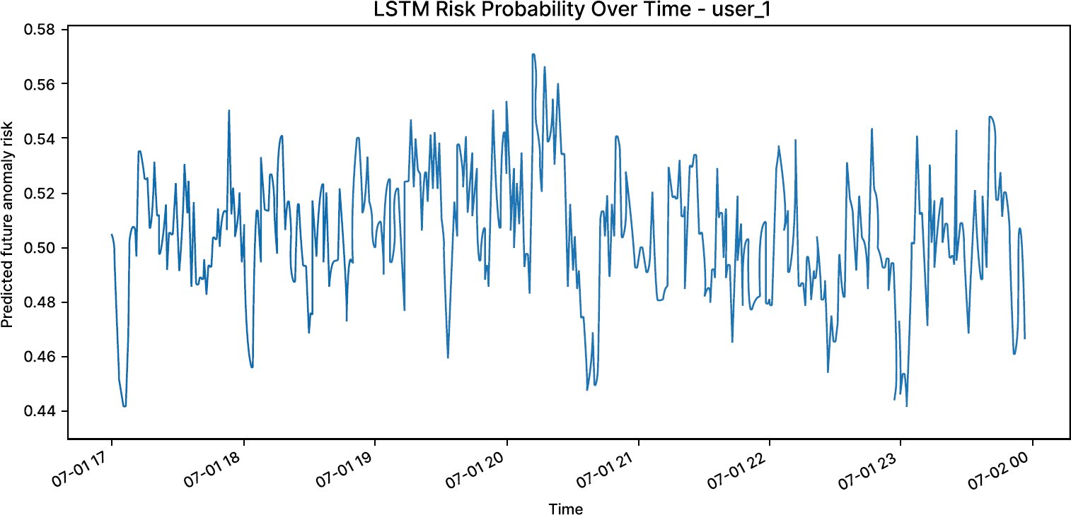
To support interpretability, SHapley Additive exPlanations (SHAP) were calculated for the final LSTM using GradientExplainer. Fifty development sequences were selected deterministically at evenly spaced indices across the 9,870 available LSTM development sequences and used as the SHAP background/reference set, while the first 200 held-out sequences were explained. GradientExplainer was executed with nsamples=50, and no held-out sequence was used in the background set. The sample size was selected as a computationally efficient approximation of the training distribution while preserving representative temporal feature variation. The resulting attribution array had shape (200, 12, 31), corresponding to sequences, time steps, and input features. Global feature importance was calculated as the mean absolute SHAP value averaged across all 200 explained sequences and all 12-time steps for each feature. A local sequence-level explanation was also produced by aggregating the 12 time-step attributions for an individual held-out sequence.
The anomaly-risk forecasting pipeline is summarised in Fig. (1). Core resource telemetry is validated, cleaned, transformed to user-specific temporal predictors, and chronologically split into a fitting, a validation and a held-out period. The type of work is also included in the context and for diagnostic and subgroup analysis, but not in the key predicting feature subset. Imbalance-sensitive as well as service-reliability measures are used to evaluate the predictive performance, and SHAP is employed to interpret the predictions of LSTM
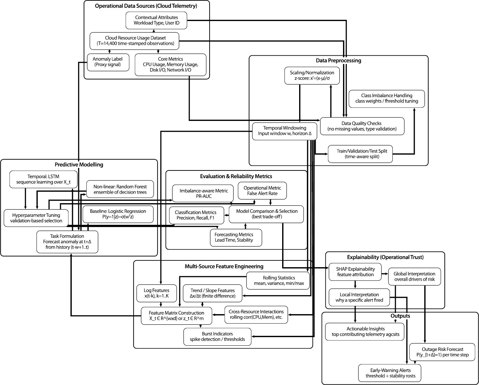
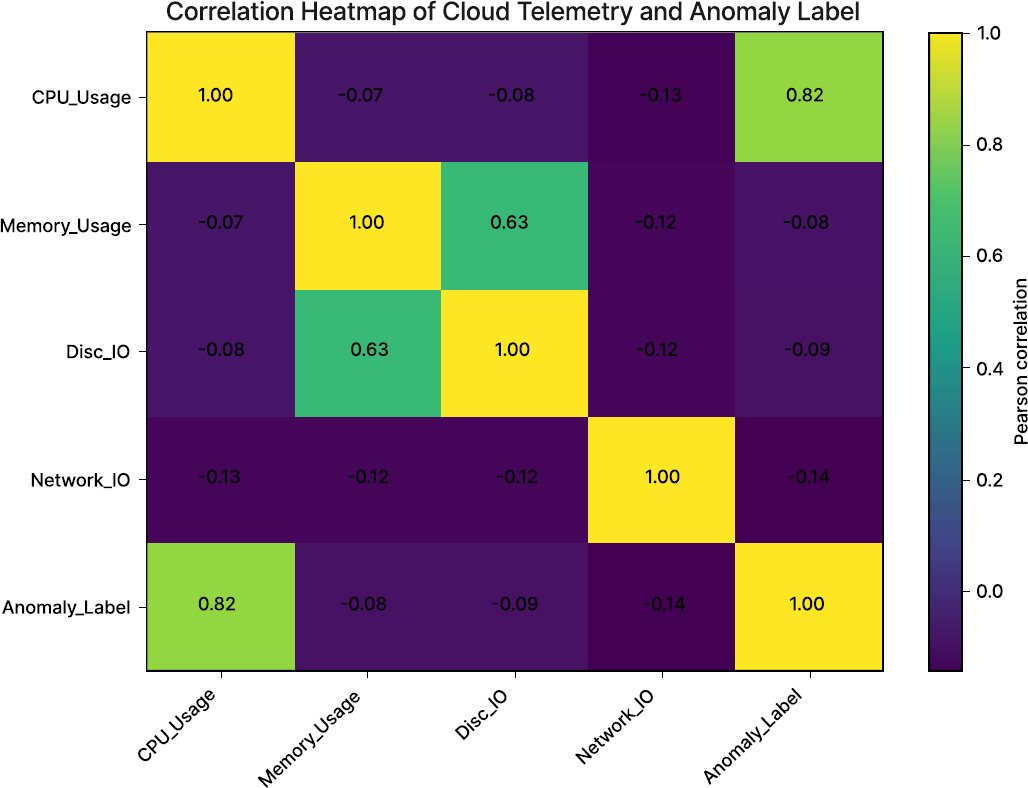
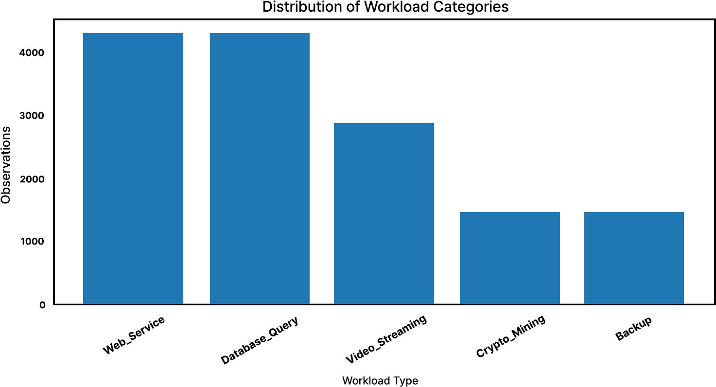
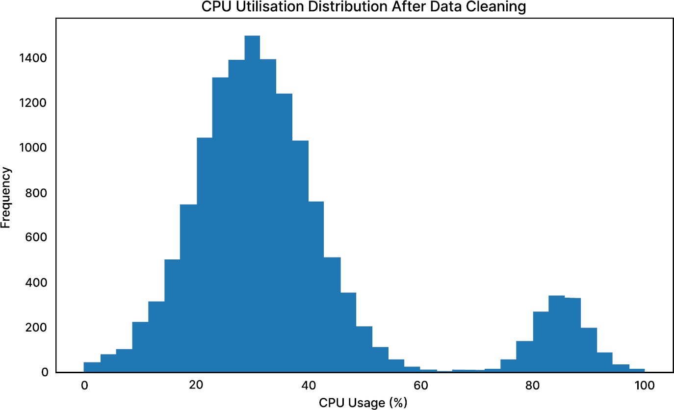
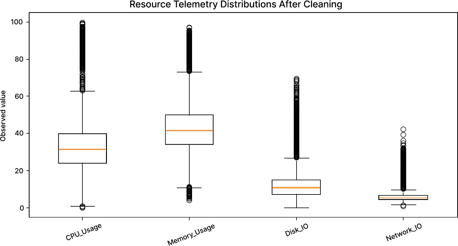
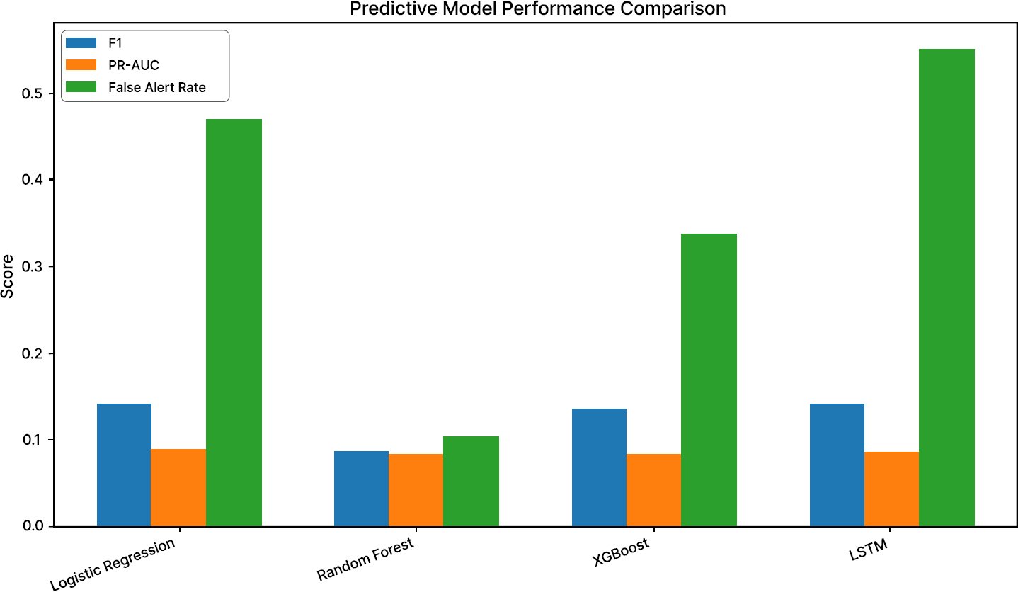
Table 4(b) results show that its contribution varies across models rather than producing a consistent improvement. For Logistic Regression, inclusion slightly increased PR-AUC from 0.0874 to 0.0890 and reduced the false-alert rate, but precision, recall, and F1 declined. Random Forest benefited most in precision, recall, and F1, with F1 increasing from 0.0859 to 0.1000, although PR-AUC marginally decreased. XGBoost also improved modestly across precision, recall, F1, and PR-AUC after workload inclusion. In contrast, LSTM performance weakened, with recall falling from 0.5513 to 0.4927 and F1 from 0.1421 to 0.1378. Overall, workload information appears more useful for tree-based models than for the linear and recurrent architectures.
Table 4(b). Workload-feature inclusion sensitivity.
| Model | Workload Feature | Precision | Recall | F1 | PR-AUC | False-Alert Rate |
| Logistic Regression | Excluded | 0.0827 | 0.4751 | 0.1408 | 0.0874 | 0.4696 |
| Logistic Regression | Included | 0.0789 | 0.4487 | 0.1343 | 0.0890 | 0.4662 |
| Random Forest | Excluded | 0.0773 | 0.0968 | 0.0859 | 0.0825 | 0.1029 |
| Random Forest | Included | 0.0888 | 0.1144 | 0.1000 | 0.0818 | 0.1045 |
| XGBoost | Excluded | 0.0837 | 0.3460 | 0.1349 | 0.0822 | 0.3372 |
| XGBoost | Included | 0.0858 | 0.3578 | 0.1384 | 0.0847 | 0.3395 |
| LSTM | Excluded | 0.0816 | 0.5513 | 0.1421 | 0.0845 | 0.5529 |
| LSTM | Included | 0.0801 | 0.4927 | 0.1378 | 0.0853 | 0.5040 |
4.5. Feature Ablation Analysis
An ablation study was conducted to determine whether predictive performance was driven mainly by the LSTM architecture or by engineered temporal features. Feature groups were removed systematically while the model architecture was kept constant. This design isolates the contribution of lag features, rolling statistics, and cross-resource interactions.
Table 5 shows small, non-monotonic ablation effects. Removing lag features increased F1 from 0.1421 to 0.1442, and removing rolling statistics increased F1 to 0.1449 and PR-AUC to 0.0893. The raw-metrics-only configuration produced F1=0.1385. Accordingly, the ablation results do not demonstrate a universal predictive gain from engineered temporal features; their principal value in this dataset may instead lie in representation diversity, cross-resource characterisation, and interpretability rather than consistent improvement in aggregate F1 or PR-AUC.
Table 5. Feature ablation study results.
| Feature Configuration | Precision | Recall | F1-Score | PR-AUC |
| Full Model (All 31 Features) | 0.0816 | 0.5513 | 0.1421 | 0.0845 |
| Without Lag Features | 0.0838 | 0.5161 | 0.1442 | 0.0846 |
| Without Rolling Statistics | 0.0845 | 0.5073 | 0.1449 | 0.0893 |
| Without Cross-Resource Features | 0.0787 | 0.4223 | 0.1327 | 0.0801 |
| Raw Metrics Only | 0.0886 | 0.3167 | 0.1385 | 0.0849 |
4.6. Robustness and Statistical Validation Results
Robustness was evaluated quantitatively using Gaussian-noise perturbation, workload-specific subgroup analysis, temporal-segment evaluation, and paired bootstrap resampling. All robustness tests used the held-out chronological test partition, and the trained Logistic Regression, Random Forest, XGBoost, and LSTM models were not re-estimated during robustness testing. Table 6 presents Gaussian-noise robustness results, Table 7(a) reports workload-specific performance, Table 7(b) presents temporal-segment robustness, Table 7(c) reports sustained-anomaly sensitivity, and Table 8 presents the paired-bootstrap comparisons between the LSTM and the baseline models.
Table 6. Gaussian-noise robustness results for all predictive models.
| Model | Precision | Recall | F1-Score | PR-AUC | False-Alert Rate | ΔF1 | ΔPR-AUC | Condition |
| Logistic Regression | 0.0852 | 0.4868 | 0.1450 | 0.0866 | 0.4657 | +0.0042 | -0.0008 | Gaussian noise |
| Random Forest | 0.0716 | 0.0850 | 0.0777 | 0.0858 | 0.0982 | -0.0082 | +0.0032 | Gaussian noise |
| XGBoost | 0.0852 | 0.3314 | 0.1355 | 0.0877 | 0.3171 | +0.0006 | +0.0054 | Gaussian noise |
| LSTM | 0.0800 | 0.5396 | 0.1393 | 0.0847 | 0.5526 | -0.0028 | +0.0002 | Gaussian noise |
Table 7(a). Workload-specific performance for all predictive models.
| Workload | Model | N | Positive | Precision | Recall | F1 | PR-AUC |
| Backup | Logistic Regression | 444 | 37 | 0.0792 | 0.4324 | 0.1339 | 0.1101 |
| Backup | Random Forest | 444 | 37 | 0.0000 | 0.0000 | 0.0000 | 0.0893 |
| Backup | XGBoost | 444 | 37 | 0.0894 | 0.2973 | 0.1375 | 0.0953 |
| Backup | LSTM | 444 | 37 | 0.0810 | 0.4595 | 0.1377 | 0.0857 |
| Crypto Mining | Logistic Regression | 399 | 31 | 0.0674 | 0.5806 | 0.1208 | 0.0702 |
| Crypto Mining | Random Forest | 399 | 31 | 0.0513 | 0.1290 | 0.0734 | 0.0788 |
| Crypto Mining | XGBoost | 399 | 31 | 0.0757 | 0.4516 | 0.1296 | 0.0700 |
| Crypto Mining | LSTM | 399 | 31 | 0.0699 | 0.6129 | 0.1254 | 0.0815 |
| Database Query | Logistic Regression | 1,293 | 115 | 0.0968 | 0.5043 | 0.1625 | 0.1050 |
| Database Query | Random Forest | 1,293 | 115 | 0.0926 | 0.1304 | 0.1083 | 0.0944 |
| Database Query | XGBoost | 1,293 | 115 | 0.0892 | 0.3739 | 0.1441 | 0.0966 |
| Database Query | LSTM | 1,293 | 115 | 0.0870 | 0.5391 | 0.1498 | 0.0973 |
| Video Streaming | Logistic Regression | 821 | 66 | 0.0826 | 0.4242 | 0.1383 | 0.0786 |
| Video Streaming | Random Forest | 821 | 66 | 0.0435 | 0.0303 | 0.0357 | 0.0799 |
| Video Streaming | XGBoost | 821 | 66 | 0.0885 | 0.2576 | 0.1318 | 0.0846 |
| Video Streaming | LSTM | 821 | 66 | 0.0813 | 0.5606 | 0.1420 | 0.0755 |
| Web Service | Logistic Regression | 1,213 | 92 | 0.0759 | 0.4565 | 0.1302 | 0.0984 |
| Web Service | Random Forest | 1,213 | 92 | 0.0876 | 0.1304 | 0.1048 | 0.0794 |
| Web Service | XGBoost | 1,213 | 92 | 0.0773 | 0.3587 | 0.1272 | 0.0802 |
| Web Service | LSTM | 1,213 | 92 | 0.0809 | 0.5761 | 0.1419 | 0.0946 |
Table 7(b). Temporal robustness results for all predictive models.
| Segment | Model | N | Positive Rate | Precision | Recall | F1 | PR-AUC |
| Early | Logistic Regression | 2,080 | 0.0822 | 0.0816 | 0.4795 | 0.1395 | 0.0854 |
| Early | Random Forest | 2,080 | 0.0822 | 0.0751 | 0.0936 | 0.0833 | 0.0807 |
| Early | XGBoost | 2,080 | 0.0822 | 0.0835 | 0.3450 | 0.1344 | 0.0831 |
| Early | LSTM | 2,080 | 0.0822 | 0.0793 | 0.5380 | 0.1382 | 0.0838 |
| Late | Logistic Regression | 2,090 | 0.0813 | 0.0838 | 0.4706 | 0.1422 | 0.0961 |
| Late | Random Forest | 2,090 | 0.0813 | 0.0794 | 0.1000 | 0.0885 | 0.0871 |
| Late | XGBoost | 2,090 | 0.0813 | 0.0840 | 0.3471 | 0.1353 | 0.0834 |
| Late | LSTM | 2,090 | 0.0813 | 0.0838 | 0.5647 | 0.1460 | 0.0874 |
Table 7(c). Sustained-anomaly sensitivity analysis.
| k | Model | Positive Prevalence | Recall | F1 | PR-AUC | False-Alert Rate | Episodes | Warning Coverage |
| 2 | Logistic Regression | 0.010072 | 0.4762 | 0.0237 | 0.0135 | 0.3937 | 21 | 0.5238 |
| 2 | Random Forest | 0.010072 | 0.0476 | 0.0430 | 0.0128 | 0.0119 | 21 | 0.0476 |
| 2 | XGBoost | 0.010072 | 0.1429 | 0.0155 | 0.0130 | 0.1756 | 21 | 0.1905 |
| 2 | LSTM | 0.010072 | 0.5238 | 0.0238 | 0.0306 | 0.4319 | 21 | 0.5238 |
| 3 | All models | 0.000000 | N/E | N/E | N/E | N/E | 0 | N/E |
| 5 | All models | 0.000000 | N/E | N/E | N/E | N/E | 0 | N/E |
4.6.1. Gaussian-Noise Robustness Test
For feature j, the perturbed test-set value was calculated as:

where  and
and  denotes the training-set standard deviation of feature
  . Zero-mean Gaussian noise equal to 10% of the feature-specific training standard deviation was added independently to the raw held-out CPU usage, memory usage, disk I/O, and network I/O values. Physical bounds were then reapplied and all lag, rolling, slope, burst, and cross-resource features were recomputed from the perturbed telemetry before scoring the already fitted models.
Gaussian-noise perturbation produced only small performance changes. F1 changed by +0.0042 for Logistic Regression, -0.0082 for Random Forest, +0.0006 for XGBoost, and -0.0028 for LSTM. PR-AUC changes were -0.0008, +0.0032, +0.0054, and +0.0002, respectively. These results indicate limited sensitivity to the specified 10% raw-telemetry perturbation, although the low clean-test discrimination remains the more important limitation.
4.7. Workload-Specific Robustness
There were 4170 forecasting observations in the common aligned chronological test set. Workload type was not a part of the principal predictor matrix in the evaluation of each observation, but was only evaluated based on the workload category known at the time of the observation. The numbers of positives in the subgroups add up to 4,170 as do the numbers of positives in the main held-out evaluation set.
For each of the various workloads, performance was different; but none of the workloads experienced the very high positive prevalence that was previously observed in the misaligned target. The percentages of positive cases for Crypto Mining, Database Query, and Database Construction were 31/399, 115/1,293, and 1,105/11,400, respectively. LSTM F1 was found to be between 0.1254 and 0.1498 across workloads, and Logistic Regression achieved a value of 0.1625 in Database Query. Random Forest was generally conservative. No universal superiority of any model is demonstrated in these results, which indicate that there is some variation in workload.
4.8. Temporal Robustness
The common aligned held-out forecasting sequences were split into two non-overlapping temporal subsets: 2080 sequences were in the early time period, and 2090 sequences were in the late time period. There were no significant differences in the positive prevalence between segments (0.0822 and 0.0813). The same fitted models and the same 0.50 thresholds were used in both segments. The performance estimates for the early and late prediction times for all four predictive models are reported in Table 7(b).
Minimal change was observed in the short timeframe results. Logistic Regression F1 changed from 0.1395 to 0.1422, Random Forest from 0.0833 to 0.0885, XGBoost from 0.1344 to 0.1353, and LSTM from 0.1382 to 0.1460. LSTM PR-AUC changed from 0.0838 to 0.0874. Such differences are not a sign of a short horizon collapse, but the set of data is still quite short, around one day, to evaluate long-term concept drift.
The results are controlled evidence of short-term temporal stability for the data that is available. In real-world cloud environments, software configurations, traffic patterns, infrastructure, and workload characteristics can evolve over a longer period, so they don’t rule out the possibility of longer-term concept drift.
In the k = 3 and k = 5 cases, there were no positive held-out observations or episodes, so the precision, recall, F1, PR-AUC, false-alert rate, and warning coverage were not estimable.
Table 7(c) indicates that the sustained-anomaly definition significantly lowered prevalence of positive events. With k = 2, there were only 42 positive observations and 21 episodes left to test the predictive performance of all four models, and with k = 3 and k = 5 there were none of the positive held-out cases to assess the models reliably.
4.9. Paired Bootstrap Confidence Intervals
The commonly held-out predictions were subject to a paired bootstrap significance test with 1,000 repetitions. On F1 and PR-AUC, LSTM was compared with Logistic Regression and Random Forest with the same resampled indices.
Bootstrap distributions were computed and the 95% confidence intervals are based on the 2.5th and the 97.5th percentiles. Empirical two-sided p-values were computed with a finite-sample correction to avoid reporting zero p-values.
Paired bootstrap resampling showed no statistically significant difference between LSTM and Logistic Regression for F1 (difference 0.0013, 95% CI [-0.0141, 0.0159], p = 0.836) or PR-AUC (difference -0.0029, 95% CI [-0.0140, 0.0062], p = 0.528). LSTM exceeded Random Forest significantly for F1 (difference 0.0562, 95% CI [0.0299, 0.0842], p = 0.002), but not for PR-AUC (difference 0.0020, p = 0.682). LSTM and XGBoost were statistically indistinguishable for F1 (difference 0.0072, p = 0.488) and PR-AUC (difference 0.0023, p = 0.724) (Table 8).
Table 8. Paired bootstrap comparison of LSTM performance against baseline models.
| Comparison | Metric | Observed Difference | 95% Confidence Interval | Two-Sided Bootstrap p-value | Significant |
| LSTM – Logistic Regression | F1 | 0.0013 | [-0.0141, 0.0159] | 0.836 | No |
| LSTM – Logistic Regression | PR-AUC | -0.0029 | [-0.0140, 0.0062] | 0.528 | No |
| LSTM – Random Forest | F1 | 0.0562 | [0.0299, 0.0842] | 0.002 | Yes |
| LSTM – Random Forest | PR-AUC | 0.0020 | [-0.0086, 0.0127] | 0.682 | No |
| LSTM – XGBoost | F1 | 0.0072 | [-0.0141, 0.0309] | 0.488 | No |
| LSTM – XGBoost | PR-AUC | 0.0023 | [-0.0103, 0.0144] | 0.724 | No |
The conclusion is thus not generalisable that the LSTM is superior. The only difference that was statistically significant among the tested differences was LSTM vs. Random Forest (F1). The differences between LSTM and all three baselines (random, most recent, and most popular) were not statistically significant at 0.05. Overall, the robustness analyses indicate moderate temporal sensitivity for short time horizons, moderate perturbation, and large differences in alerting trade-offs between models and workloads, and limited discrimination. These analyses are helpful to the internal diagnostic process but cannot replace longer-duration, independently labelled production telemetry.
4.10. Explainability Results
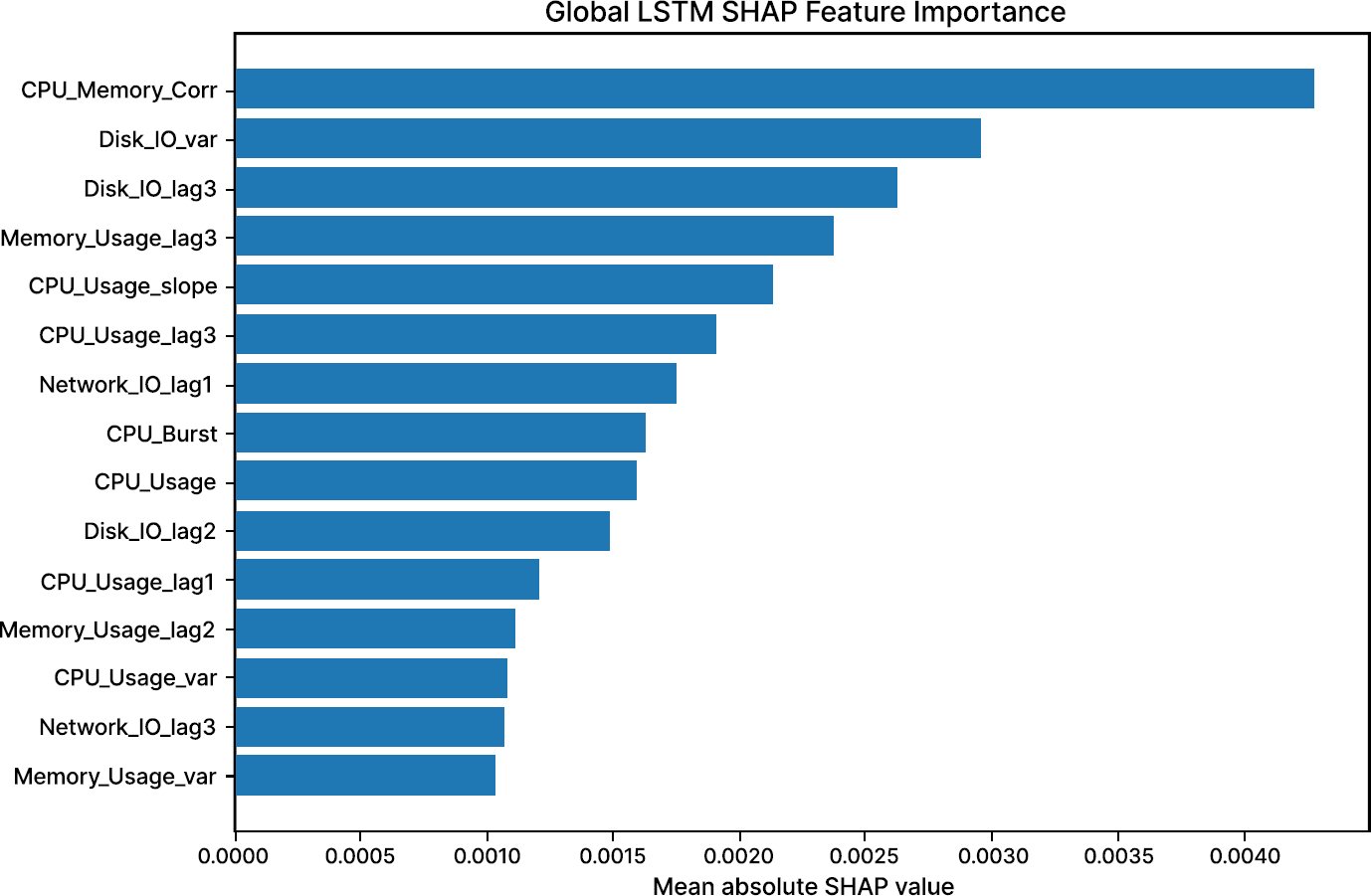
The final SHAP GradientExplainer analysis was successfully carried out on 200 test sequences of LSTM, resulting in an attribution array of shape (200, 12, 31). Global mean absolute SHAP importance, averaged across all 200 sequences and 12 time steps, ranked CPU_Memory_Corr first (0.004278), followed by Disk_IO_var (0.002954), Disk_IO_lag3 (0.002615), Memory_Usage_lag3 (0.002381), CPU_Usage_slope (0.002136), and CPU_Usage_lag3 (0.001908). The explanation thus suggests a representation of a mixed cross-resource and temporal mechanism, not just a mechanism dominated by CPU saturation.
Fig. (7) shows that both cross-resource dependence and lagged/variability terms contribute to the LSTM risk score. CPU_Memory_Corr was the strongest global feature, while disk variance, disk lag 3, memory lag 3, and CPU slope also ranked highly. These attributions improve transparency but should be interpreted as model explanations for this dataset rather than causal evidence of operational failure mechanisms.
Licensed
© 2026 Copyright by the Authors.
Licensed as an open access article using a CC BY 4.0 license.