


















Article Contents
Article ID: CM2601105009
Views: 36Leveraging Artificial Intelligence for Smart Retail Decision Support: A Proof-of-Concept Framework for Demand Forecasting, Inventory Simulation, and Synthetic Workflow Assignment
 DOI:
 PDF
⬇ Downloads: 3
1NED University of Engineering and Technology, Karachi, Pakistan
Received: 01 September, 2026
Revised: 01 October, 2026
Accepted: 06 October, 2026
Published: 21 October, 2026
ABSTRACT
Introduction: This study presents a proof-of-concept smart-retail decision-support framework that links demand forecasting, fixed-threshold inventory simulation, and trigger-gated synthetic workflow assignment.
Methodology: An exploratory ItemID 1 analysis reports in-sample RMSE and MAE for Prophet, ARIMA, XGBoost, and LSTM as model-fit diagnostics only. A separate Store 1–Item 1 LSTM, trained with a chronological 90/10 split and training-only scaling, produces 182 one-step-ahead outputs for 3 July–31 December 2017, which serve as demand inputs to the inventory simulation.
Results: This demand path, a 30-unit reorder threshold gave a lower average inventory level (81.68 versus 98.71 units) and a lower simulated holding-cost component ($1,486.60 versus $1,796.60) than a 50-unit threshold. A deterministic synthetic workflow releases an officer assignment only when a procurement trigger occurs.
Conclusion: The contribution is the explicit orchestration of interfaces from forecasting output to replenishment events and gated task assignment. The evidential scope of each component is reported separately, and the results are not evidence of forecasting superiority, optimal inventory policy, or operational performance.
Keywords: Artificial intelligence, smart retail, demand forecasting, inventory simulation, fixed-threshold replenishment, synthetic workflow assignment, robotic process automation, decision tree classification, proof of concept.
1. INTRODUCTION
Retail demand is increasingly volatile while supply-chain processes are becoming more digitalised and tightly coupled, making timely demand information, inventory visibility, and coordinated execution increasingly important [1–4]. Forecast uncertainty can affect replenishment decisions, while slow or disconnected workflows can delay operational action. The value of Artificial Intelligence (AI) in this setting therefore depends not only on generating model outputs but also on connecting those outputs to inventory and workflow decisions.
Retail planning commonly separates forecasting, inventory control, and task allocation. Inventory modelling provides reference points for replenishment rules and cost-sensitive stock dynamics, including models for deteriorating items, variable demand, holding costs, shortages, and backlogging [5]. AI-enabled forecasting and smart-retail studies more directly examine how demand information can support downstream inventory decisions [6–8]. These methods provide useful reference points for examining how forecasting information can be connected to downstream inventory and workflow decisions. This study therefore investigates a connected decision-support pipeline while keeping exploratory forecasting evidence, inventory simulation, and the synthetic workflow demonstration analytically distinct.
This study presents a modular proof-of-concept implementation for retail decision support rather than a validated production system. Public retail data and a separate Store 1–Item 1 LSTM implementation demonstrate three connected components: (i) In-sample fitted-error diagnostics for Prophet, ARIMA, XGBoost, and LSTM on ItemID 1; (ii) An inventory simulation that compares two fixed reorder thresholds using Store 1–Item 1 LSTM outputs as demand inputs; and (iii) A synthetic workflow in which procurement-trigger events activate synthetic officer assignments. Four terms are used throughout. ‘Exploratory four-model analysis’ denotes the in-sample diagnostics on ItemID 1. ‘Store 1–Item 1 LSTM’ denotes the separate, chronologically split implementation that supplies demand inputs to the inventory simulation. ‘Configuration A’ and ‘Configuration B’ denote the 30-unit and 50-unit reorder thresholds, respectively. ‘Synthetic workflow layer’ denotes the task-assignment demonstration based on simulated features and synthetic officer labels. No production Robotic Process Automation (RPA) bot is implemented; RPA is discussed only as a possible downstream execution mechanism.
Two public Kaggle datasets are used for separate analyses. The Demand Forecast for Optimized Inventory Planning dataset supplies ItemID 1 for the exploratory Prophet, ARIMA, XGBoost, and LSTM model-fit demonstration. The Store-Item Demand Forecasting challenge separately supplies Store 1–Item 1 for the LSTM, inventory, and workflow implementation. Synthetic workflow labels are generated within the implementation and are not drawn from either retail dataset.
The primary contribution is architectural and integrative rather than algorithmic. First, the exploratory four-model component characterises in-sample model fit. Second, the Store 1–Item 1 LSTM provides a dated stream of model-generated demand inputs to a fixed-threshold replenishment simulation. Third, procurement-trigger events from the inventory layer gate the release of synthetic task-assignment outputs. The orchestration contribution therefore lies in the explicit interfaces between model output, replenishment logic, and event-driven workflow activation. This positioning is consistent with work connecting forecasting and inventory decisions [7, 8] and with procurement research on RPA and process automation [9, 10].
The remainder of the paper is organised as follows. The Method section includes information about the datasets used, the forecasting procedure, inventory assumptions, the synthetic workflow design, and analytical methods. The Results and Analysis section presents forecasting and inventory-simulation as well as the synthetic workflow. The Discussion provides an interpretation of these results in the context of past studies and the suggested proof-of-concept study framework, limitations, future validations needed, and conclusions.
2. METHODOLOGY
The methodology consists of an exploratory forecasting component, a controlled fixed-threshold inventory simulation, and a synthetic workflow-classification demonstration. The three modules do not share a single enterprise dataset; instead, they are connected through a common decision flow. Synthetic procurement labels are generated independently of the sales datasets, as illustrated in Fig. (1), and module-level feasibility is not treated as evidence of production deployment.
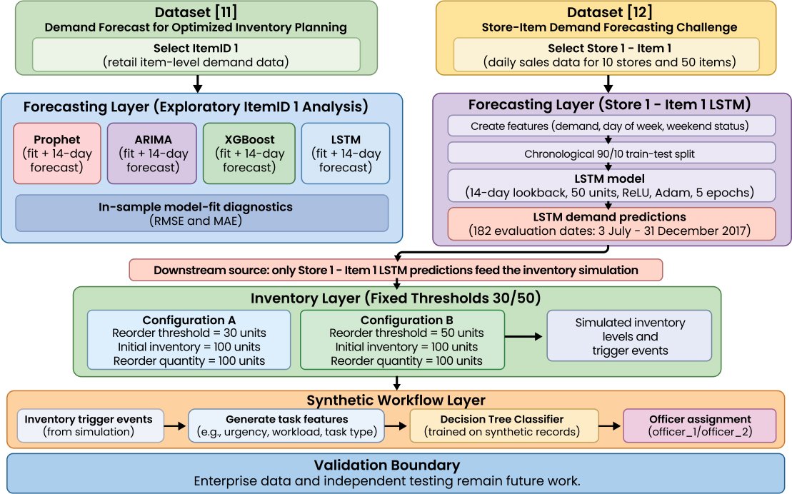
Fig. (1). Proof-of-concept methodology and data provenance.
2.1. Dataset Description
Two public retail datasets support separate analytical components. The Demand Forecast for Optimized Inventory Planning dataset [11] supplies ItemID 1 for the exploratory Prophet, ARIMA, XGBoost, and LSTM model-fit comparison. The Store-Item Demand Forecasting Challenge [12], which contains daily sales from 1 January 2013 to 31 December 2017 across 10 stores and 50 items, separately supplies Store 1–Item 1 for the LSTM, inventory, and synthetic workflow implementation. The datasets are not pooled into a common forecasting benchmark.
A chronological split is used only in the Store 1–Item 1 LSTM implementation. Targets are kept in date order: the first 90% form the training segment, and the remaining 10% (182 daily targets, 3 July–31 December 2017) form the held-out segment. Each target is predicted from a 14-day window of observed lagged inputs (demand, day-of-week, and weekend status). Prediction is sequence-to-one and one-step-ahead; earlier predictions are not fed back into later windows, so the procedure is not a free-running recursive 182-day forecast. MinMax scaling parameters are fitted exclusively on training-period values and applied unchanged to held-out inputs, and the inverse transformation uses the training-fitted demand scale. All random seeds were fixed (seed = 42) with deterministic TensorFlow operations, and the LSTM was trained once the same 182 outputs feed the inventory simulation and the workflow demonstration.
2.2. Evaluation Units
The two forecasting implementations use different datasets, predictors, and evaluation designs. The exploratory component (dataset [11], ItemID 1) reports in-sample fitted errors and illustrative 14-day future forecasts, whereas the Store 1–Item 1 component (dataset [12]) supplies the 182 held-out outputs. Their results are therefore not combined into a common out-of-sample ranking of Prophet, ARIMA, XGBoost, and LSTM.
2.3. Forecasting Implementations
Prophet, ARIMA, XGBoost, and LSTM were selected to represent additive time-series, classical statistical, tree-based machine-learning, and recurrent neural-network approaches, respectively. The implementation details below follow the actual notebook and are not presented as a common out-of-sample test-set benchmark.
The implementation contains an exploratory four-model component and a separate Store 1–Item 1 LSTM component. In the exploratory ItemID 1 analysis, Prophet is fitted with daily seasonality enabled and produces fitted values together with a 14-day future forecast, consistent with established Prophet methodology and retail application [13, 14]. ARIMA is implemented as ARIMA (5,1,0), providing a classical statistical comparator with established retail-forecasting use [15]. XGBoost uses XGBRegressor with a squared-error regression objective and a sequential day-index predictor. The exploratory LSTM uses a five-observation sequence length, 50 recurrent units with ReLU activation, one dense output unit, Adam optimisation, mean-squared-error loss, and 10 epochs. Error measures from this component are calculated on fitted observations and are interpreted only as in-sample model-fit diagnostics.
The separate Store 1–Item 1 LSTM uses demand, day-of-week, and weekend-status features with a 14-day lookback. The network has 50 LSTM units with ReLU activation, one dense output unit, Adam optimisation, mean-squared-error loss, five epochs, and a batch size of 32. Inverse-transformed held-out outputs are used as demand inputs for the inventory simulation.
The implementation notebook is provided as Supplementary Material to support reproducibility. No inferential pairwise comparison among the four forecasting models is performed.
2.4. Model Hyperparameters and Training Configuration
Table 1 summarises the configurations actually implemented in the accompanying notebook. The exploratory and Store 1–Item 1 LSTM components are shown separately because they use different datasets and model settings.
Table 1. Forecasting configurations implemented in the notebook.
| Component | Implemented Configuration |
| Exploratory Prophet | ItemID 1; Prophet with daily seasonality enabled; fitted values plus 14-day future forecast |
| Exploratory ARIMA | ItemID 1; ARIMA (5,1,0); fitted values plus 14-day future forecast |
| Exploratory XGBoost | ItemID 1; XGBRegressor; objective = reg:squarederror; sequential day index predictor; fitted values plus 14-day future forecast |
| Exploratory LSTM | ItemID 1; sequence length = 5; 50 LSTM units; ReLU; Dense (1); Adam; MSE; 10 epochs |
| Store 1–Item 1 LSTM | demand + day-of-week + weekend features; lookback = 14; chronological 90/10 split; MinMax scaler fitted on training segment only; held-out chronological sequence-to-one prediction (observed lag windows; non-recursive); 50 LSTM units; ReLU; Dense (1); Adam; MSE; 5 epochs; batch size = 32; random seed = 42 |
2.5. Inventory Simulation Parameters
The inventory component applies a simple fixed-threshold simulation to the 182 Store 1–Item 1 LSTM demand predictions. Both configurations begin with 100 units of stock and replenish by 100 units. Configuration A reorders when inventory is at or below 30 units, whereas Configuration B reorders at or below 50 units. Because both configurations use the same demand path and differ only in the reorder threshold, the comparison is a threshold-sensitivity demonstration rather than a comparison of forecasting-model performance or a formal inventory-optimisation study.
For each LSTM-generated demand input, demand is subtracted from the current simulated inventory balance. If the arithmetic balance falls below zero, the implementation records a negative-inventory event. This term is deliberately distinguished from a stockout. The simulation does not explicitly model unmet demand, lost sales, backorders, fill rate, or cycle service level, so a negative balance cannot be interpreted as a validated stockout or service-failure measure. Formal EOQ, safety stock, supplier lead time, and ordering cost are also not implemented. Holding cost is assumed to be $0.10 per unit per evaluation day, and the implemented negative-inventory-event penalty is $2.00 per event. Average inventory is the mean opening balance over the 182 steps, and the holding-cost component equals this average multiplied by $0.10 and by the 182 evaluation days.
Table 2 summarises the implemented settings. The reorder threshold is the only manipulated parameter.
Table 2. Inventory parameters implemented in the notebook.
Parameter | Configuration A | Configuration B |
Demand input | LSTM-generated demand inputs | LSTM-generated demand inputs |
Held-out LSTM outputs / inventory steps | 182 | 182 |
Evaluation dates | 3 July–31 December 2017 | 3 July–31 December 2017 |
Initial inventory | 100 | 100 |
Reorder quantity | 100 | 100 |
Reorder threshold | 30 | 50 |
Holding-cost assumption | $0.10/unit/day | $0.10/unit/day |
Negative-inventory-event penalty | $2.00/event | $2.00/event |
Formal EOQ | Not implemented | Not implemented |
Lead time | Not modelled | Not modelled |
Safety stock | Not modelled | Not modelled |
2.6. Inventory Simulation and Fair-Comparison Boundary
The simulation uses the complete held-out segment: 182 daily LSTM outputs for 3 July–31 December 2017, each supplying one demand input to one inventory step. The same 182 inputs are applied to both configurations. Fig. (2) shows the resulting trajectories, and Table 3 reports the descriptive outputs.
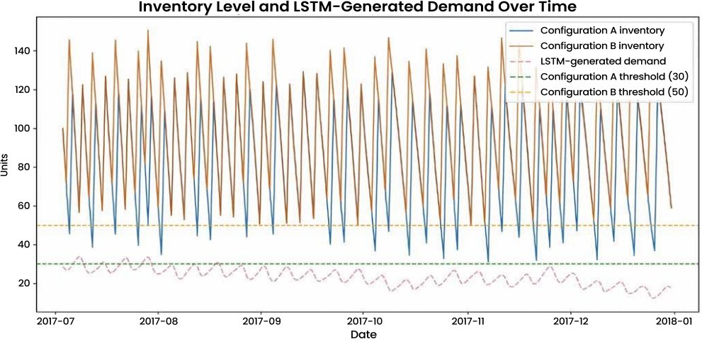
Fig. (2). LSTM-generated demand and inventory trajectories for the two fixed-threshold configurations.
Table 3. Descriptive outputs of the two implemented replenishment configurations.
| Measure | Configuration A | Configuration B |
| Reorder threshold | 30 units | 50 units |
| Initial inventory | 100 units | 100 units |
| Reorder quantity | 100 units | 100 units |
| Average inventory | 81.68 units | 98.71 units |
| Recorded negative-inventory events | 0 | 0 |
| Holding-cost assumption | $0.10/unit/day | $0.10/unit/day |
| Simulated holding cost | $1,486.60 | $1,796.60 |
| Negative-inventory-event penalty cost | $0.00 | $0.00 |
| Partial simulated cost | $1,486.60 | $1,796.60 |
Note: The monetary values are partial simulated cost components (holding cost plus the $2.00 negative-inventory-event penalty) and exclude ordering cost; they are not total inventory costs. A negative-inventory event records an arithmetic balance below zero. Because unmet demand, lost sales, backorders, fill rate, and lead-time service are not modelled, zero recorded events do not imply zero stockouts or validated service performance.
2.7. Synthetic Workflow Classifier Demonstration
The synthetic workflow uses item type, urgency, workload_officer1, and workload_officer2 as demonstration features. The target label is deterministic: officer_1 is assigned when workload_officer1 is lower than workload_officer2, and officer_2 otherwise. The two workload variables are generated as integers from 1 to 4 with random seed 42, and item type is drawn at random from A, B, and C. Urgency is set to 1 when LSTM-generated demand exceeds 80 units and to 0 otherwise. Because the same simulated workload variables define the target and are provided to the decision tree, the classifier reproduces a pre-programmed rule rather than learning employee effectiveness. The tree is fitted to and illustrated with the same synthetic records, so no accuracy, precision, recall, F1-score, confusion-matrix, or workforce-effectiveness claim is made. External validation would require observed procurement, workload, staff-availability, skill, lead-time, purchase-order, and task-outcome data.
The 80-unit urgency cut-off is a fixed, illustrative priority rule that was set a priori in the same units as the 100-unit reorder quantity; it was not estimated from the data. In the held-out segment, LSTM-generated demand ranges from 12.5 to 34.1 units (the maximum daily sales in the full Store 1–Item 1 series is 50 units), so no row exceeds the cut-off. Urgency is therefore 0 in all 182 rows and has no influence on the synthetic labels, which is why the demand values in Table 4 lie far below 80. The flag is retained only to show where a priority variable would enter the workflow. In applied use, the cut-off should be calibrated to business priorities or a high percentile of observed demand and tested on data in which urgent cases occur.
Table 4. Sample synthetic workflow outputs with trigger-gated assignments (last ten evaluation dates).
| Date | Demand | Inventory Level | Triggered | Item Type | Officer Output |
| 2017-12-22 | 17.95 | 83.75 | No | C | Not activated |
| 2017-12-23 | 18.14 | 65.61 | No | B | Not activated |
| 2017-12-24 | 16.25 | 49.36 | No | C | Not activated |
| 2017-12-25 | 12.46 | 36.90 | No | A | Not activated |
| 2017-12-26 | 12.61 | 24.29 | Yes | C | officer_1 |
| 2017-12-27 | 14.12 | 110.17 | No | B | Not activated |
| 2017-12-28 | 15.45 | 94.71 | No | A | Not activated |
| 2017-12-29 | 17.29 | 77.42 | No | A | Not activated |
| 2017-12-30 | 18.44 | 58.98 | No | A | Not activated |
| 2017-12-31 | 17.56 | 41.42 | No | C | Not activated |
The decision tree can calculate a latent synthetic officer label for every demonstration row, including rows on which no procurement trigger occurs. However, the event-driven workflow activates a procurement task and exposes an officer assignment only when Triggered = Yes. Table 4 therefore reports ‘Not activated’ on non-trigger dates rather than displaying the latent label.
2.8. Workflow Automation Strategy
The workflow is a controlled synthetic layer. At each inventory step, the reorder condition is evaluated first. When the threshold is reached or crossed, a procurement task is activated and the decision-tree output is released as the synthetic officer assignment. Otherwise, no task or assignment is activated, even though the classifier can generate a latent label. No production RPA bot, real employee database, or live purchase-order system is implemented or tested.
3. RESULTS AND ANALYSIS
3.1. Forecasting Results
Two separate forecasting analyses are reported. The first uses all available ItemID 1 observations from the Demand Forecast for Optimized Inventory Planning dataset to fit Prophet, ARIMA, XGBoost, and LSTM. The resulting RMSE and MAE values are in-sample fitted-error diagnostics, not forecast-accuracy estimates, and are listed in Appendix A (Table A1) for illustration only. Each exploratory model also produces an illustrative 14-day future forecast, which is not used for any accuracy ranking.
The fitted errors differ widely across the four models (Table A1). In particular, the near-zero XGBoost error (approximately 0.001) arises because the model is evaluated on the same observations used to estimate it, with a sequential day index as its only predictor. It should not be read as forecasting accuracy.
The second implementation, the Store 1–Item 1 LSTM, produces 182 one-step-ahead outputs for the held-out dates (3 July–31 December 2017), each generated from the corresponding observed 14-day window. These outputs are passed one-for-one to the 182 inventory steps and the workflow demonstration. Prophet, ARIMA, and XGBoost are not evaluated on this segment, so no cross-model ranking on a commonly held-out horizon is available.
3.2. Inventory Simulation Results
Fig. (2) displays the Store 1–Item 1 LSTM-generated demand inputs together with the inventory trajectories produced by the two replenishment configurations across the 182-date held-out chronological segment used for downstream simulation. Configuration A uses a 30-unit reorder threshold and Configuration B uses a 50-unit threshold, with both configurations starting at 100 units and replenishing by 100 units when their respective thresholds are reached.
Both configurations use the same 182 LSTM-generated demand inputs. Configuration A (30-unit threshold) has an average simulated inventory level of 81.68 units, and Configuration B (50-unit threshold) has 98.71 units. Under the assumption of $0.10 per unit per evaluation day, the simulated holding-cost components are $1,486.60 and $1,796.60, respectively, so the lower threshold produces the lower holding-cost component in this simplified simulation. Configuration A triggers 42 procurement events and Configuration B triggers 43. No negative-inventory events are recorded for either configuration (Table 3). Across five additional random seeds, the ordering of the two configurations was unchanged (average inventory 79.5–80.5 units for A and 97.5–100.6 units for B), although one run recorded a single negative-inventory event for Configuration A. The event count therefore depends on the trained model and is not a stockout or service-level measure.
3.3. Workflow Automation Insights
The workflow experiment demonstrates the technical feasibility of converting simulated inventory events into synthetic task-assignment decisions; operational efficiency and staffing benefits are not evaluated. The decision tree uses encoded item type, a synthetic urgency indicator, workload_officer1, and workload_officer2 as predictors and produces a candidate label of officer_1 or officer_2. A separate trigger gate determines whether that label is activated as an assignment. The classifier does not predict the number of officers required.
The workflow trigger is event-driven and based on simulated inventory state; no operational latency is measured. A procurement trigger becomes active when the simulated inventory level reaches or falls below the relevant reorder threshold. Only at that point is the candidate decision-tree label released as the synthetic officer assignment. Fig. (3) illustrates this rule by plotting simulated inventory (before replenishment) against the 30-unit threshold of Configuration A and marking the 42 procurement-trigger events.
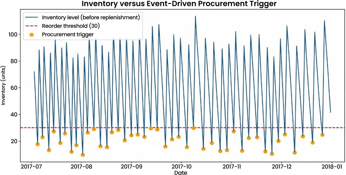
Fig. (3). Inventory versus event-driven procurement trigger.
Table 4 shows the last ten synthetic workflow rows after applying the trigger gate. Rows with Triggered = No do not create a procurement task and are shown as ‘Not activated’, whereas rows with Triggered = Yes display the synthetic officer_1 or officer_2 output. The demand values shown (12.5–18.4 units) lie far below the 80-unit urgency cut-off, so urgency is 0 in every row (see Method). The labels derive from simulated features and are not evidence that a particular officer is better suited to an item type, nor of workforce-allocation effectiveness.
The synthetic workflow thus demonstrates an event-driven task-generation concept related to RPA principles in the procurement-automation literature. Inventory events determine whether a procurement task is activated, and the decision tree supplies a synthetic officer label only for activated tasks.
4. DISCUSSION
4.1. Interpretation of Key Findings
The implementation provides three forms of proof-of-concept evidence with different methodological boundaries. First, the ItemID 1 four-model exercise provides in-sample fitted-error diagnostics (Appendix A) that do not support an out-of-sample comparison of the models. The separate Store 1–Item 1 LSTM uses training-only preprocessing and a held-out chronological segment that yields 182 one-step-ahead outputs for the downstream components.
Second, the inventory experiment varies only the reorder threshold. The 30-unit threshold yields a lower average inventory level and holding-cost component than the 50-unit threshold, which is a threshold-sensitivity result rather than evidence of lower total cost or better service. The zero values in Table 3 are negative-inventory event counts from the arithmetic balance rule, not validated stockout outcomes.
Third, the workflow element shows how procurement-trigger events can activate synthetic task-assignment outputs. Because the officer target is derived deterministically from simulated workloads and the classifier is illustrated on its own training records, the workflow demonstrates reproduction and gating of a synthetic rule, not assignment performance. Taken together, the results support a modular proof of concept rather than an end-to-end measure of operational performance.
4.2. Comparison with Previous Research
Previous research provides useful component-level reference points for positioning the framework. Yang et al., [8] integrate sensor feedback, demand forecasting, and inventory optimisation through multi-agent deep reinforcement learning, while Singhal et al., [7] connect machine-learning demand prediction with smart-retail inventory management. In procurement, Picoli and Bin [9] and Santos et al., [10] analyse RPA and RPA/BPM integration using organisational process evidence. Forecasting studies [16, 17 ,18] and methodological sources for XGBoost and recurrent neural networks [19, 20] inform the individual modelling choices used here. The present contribution is different: it provides a lightweight orchestration of an exploratory forecasting component, a separate LSTM-driven inventory simulation, and a trigger-gated synthetic workflow layer. It does not introduce a new forecasting, inventory, or classification algorithm and avoids overstating algorithmic originality or deployment readiness.
4.3. Proposed Framework
Fig. (4) presents the three-layer proof-of-concept architecture. The forecasting layer contains the exploratory ItemID 1 four-model fitted-error analysis and the separate Store 1–Item 1 LSTM. Only the 182 outputs from the LSTM held-out chronological segment feed the downstream inventory layer. The inventory layer applies the 30-unit and 50-unit fixed thresholds to the same model-generated demand path and produces procurement-trigger events. In the synthetic workflow layer, the decision tree supplies a candidate officer label, but the label is activated as an assignment only when a procurement trigger occurs. The architecture therefore represents explicit interfaces among forecasting output, replenishment logic, and workflow assignment rather than a single statistically validated end-to-end model.
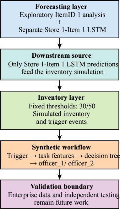
Fig. (4). Proposed proof-of-concept framework.
The architecture is modular and could support future feedback and retraining, but no live closed-loop retail deployment is tested. Scalability, latency, system integration, and operational responsiveness are not measured. Fig. (4) should therefore be interpreted as a design framework for subsequent validation rather than as evidence of current production capability.
4.4. Future Research Opportunities
The principal limitations arise from the proof-of-concept design and the different evidential bases of the three components. The four-model ItemID 1 values are in-sample fitted errors and do not test cross-model superiority out of sample. The Store 1–Item 1 LSTM is a single-series demonstration whose 182 outputs are one-step-ahead predictions from observed lagged windows rather than a recursive 182-day forecast, and its inventory results vary slightly with the random seed. The inventory simulation uses simplified fixed thresholds and omits formal EOQ, lead time, safety-stock optimisation, ordering cost, unmet-demand units, and service-level measures. Workflow labels and officer workloads are synthetic, the 80-unit urgency cut-off is an uncalibrated placeholder that is never exceeded in these data, and the classifier is not evaluated on an independent holdout set.
Future validation should preserve training-only preprocessing while evaluating Prophet, ARIMA, XGBoost, and LSTM on the same independent forecast horizon. Inventory studies should incorporate enterprise-calibrated ordering and holding costs, lead times, safety stock, order-event logs, unmet-demand measures, fill rate, and service-level outcomes. Workflow validation should use observed procurement records, employee workloads, availability and skill data, and task outcomes on a separate evaluation set, with urgency rules calibrated to observed demand. These steps are required before the framework can support defensible claims about forecasting generalisation, inventory economics, service performance, or workforce effectiveness.
CONCLUSION AND FUTURE DIRECTIONS
This study proposes a modular proof-of-concept framework linking forecasting, simplified inventory simulation, and synthetic workflow assignment. The ItemID 1 exercise reports in-sample fitted-error diagnostics rather than a common out-of-sample benchmark. A separate Store 1–Item 1 LSTM, trained on a chronological 90% split with a 14-day lookback and training-only scaling, produces 182 held-out one-step-ahead outputs (3 July–31 December 2017) that are passed one-for-one to the inventory and workflow components.
On this demand path, Configuration A (30-unit threshold) has an average inventory level of 81.68 units and a simulated holding-cost component of $1,486.60, whereas Configuration B (50-unit threshold) has 98.71 units and $1,796.60. The lower threshold therefore yields lower simulated holding cost under the stated assumptions. No claim is made about total inventory cost or service performance.
The workflow component shows how inventory triggers can activate procurement tasks and synthetic officer assignments; non-trigger rows are not assigned. Because the labels and workloads are synthetic and the same records are used for fitting and illustration, the results do not indicate predictive accuracy, workforce effectiveness, fairness, or production-RPA performance.
The primary contribution is architectural rather than algorithmic or operational: forecasting outputs, replenishment logic, and trigger-gated task assignment are orchestrated through explicit interfaces while the evidential boundary of each component is preserved. Claims about model superiority, inventory optimisation, total cost, service performance, or workforce effectiveness would require a common independent forecast horizon, enterprise-calibrated inventory parameters with complete order and unmet-demand logs, and workflow validation using observed procurement-workforce data.
LIST OF ABBREVIATIONS
| AI | = | Artificial Intelligence |
| RPA | = | Robotic Process Automation |
AUTHOR’S CONTRIBUTION
M.J. was responsible for conceptualisation, methodology, data preparation, forecasting-model development, inventory-simulation design, formal analysis, workflow-automation design, visualisation, interpretation of results, and preparation of the manuscript. The author reviewed the final version of the manuscript and approved it for submission.
ETHICAL APPROVAL & INFORMED CONSENT
Ethical approval was not required because the study uses publicly available retail datasets and synthetically generated workflow records and involves no human participants, interventions, or personally identifiable information.
AVAILABILITY OF DATA AND MATERIALS
Data Availability Statement
The public datasets used in this study are available through Kaggle as cited in References [11] and [12]. Dataset [11] supports the exploratory ItemID 1 forecasting demonstration, while dataset [12] supports the Store 1–Item 1 LSTM, inventory, and workflow implementation. The procurement-workflow records are synthetically generated within the implementation.
Code Availability Statement
The implementation notebook (Python.ipynb) is provided as Supplementary Material. It contains the fixed random seeds, training-only scaling, simulation code, and the code that generates Fig. (2) and (3) and Tables (3 and 4). It requires the public datasets cited in References [11] and [12].
The publicly available FitBit Fitness Tracker Data dataset used in this study is available through Kaggle at https://www.kaggle.com/datasets/arashnic/fitbit. The source files used in the analysis are identified in Section III-A, and no new personal data were collected by the authors.
FUNDING
This study received no external funding.
CONFLICT OF INTEREST
The author declares no conflict of interest.
ACKNOWLEDGEMENTS
The author thanks the providers of the publicly available datasets used in this proof-of-concept study.
DECLARATION OF AI
No Artificial Intelligence (AI) tools were used in the preparation of this manuscript.
APPENDIX A.
In-Sample Fitted-Error Diagnostics (ItemID 1)
Table A1 reports fitted errors calculated on the same ItemID 1 observations used to estimate the models. The values illustrate in-sample model fit only; they are not forecast-accuracy estimates and do not rank the models out of sample. The near-zero XGBoost error reflects fit to the estimation data and must not be interpreted as forecasting performance.
Table A1. Illustrative In-sample fitted-error diagnostics (not forecast accuracy) for ItemID 1
| Model | RMSE | MAE |
| Prophet | 41.405 | 18.122 |
| ARIMA | 69.100 | 36.156 |
| XGBoost | 0.001 | 0.001 |
| LSTM | 46.746 | 11.285 |
REFERENCES
[1] S. Motamary, “Implementing artificial intelligence-powered predictive maintenance and inventory forecasting in retail supply chains,” in Intelligent Retail and Manufacturing Systems: Artificial Intelligence-Driven OSS/BSS Solutions and Infrastructure Innovations. 2025, pp. 62–81,
https://doi.org/10.70593/978-93-49910-26-3_4
[2] O. R. Amosu, P. Kumar, Y. M. Ogunsuji, S. Oni, and O. Faworaja, “AI-driven demand forecasting: Enhancing inventory management and customer satisfaction,” World Journal of Advanced Research and Reviews, vol. 23, no. 2, pp. 708–719, 2024,
https://doi.org/10.30574/wjarr.2024.23.2.2394
[3] S. R. Adapa, “Optimizing supply chain efficiency through AI-driven demand forecasting: An empirical analysis of retail industries,” Library Progress International, vol. 44, no. 3, pp. 20766–20781, 2024,
https://doi.org/10.48165/bapas.2024.44.2.1
[4] V. P. Prabu, “The impact of real-time data analytics on retail supply chain efficiency,” International Journal of Innovative Research and Creative Technology, vol. 7, no. 3, pp. 1–9, 2021,
https://doi.org/10.5281/zenodo.15155661
[5] S. Rabiu and M. K. M. Ali, “Optimizing inventory dynamics: A smart approach for non-instantaneous deteriorating items with linear time function dependent variable demands and holding costs, shortages with backlogging,” Journal of Applied Mathematics and Computing, vol. 70, no. 4, pp. 3193–3217, 2024,
https://doi.org/10.1007/s12190-024-02089-1
[6] T. Ogunyankinnu, A. A. Osunkanmibi, E. F. Onotole, C. E. Ukatu, O. A. Ajayi, and Y. Adeoye, “AI-powered demand forecasting for enhancing JIT inventory models,” Journal of Frontiers in Multidisciplinary Research, vol. 5, no. 1, pp. 184–196, 2024,
https://doi.org/10.54660/.IJFMR.2024.5.1.184-196
[7] K. Singhal, V. Singh, and A. Kaul, “Smart retail: Utilizing machine learning for demand prediction, price strategy, and inventory management,” in Proc. 2024 IEEE 16th Int. Conf. Computational Intelligence and Communication Networks (CICN), 2024, pp. 485–489,
https://doi.org/10.1109/CICN63059.2024.10847534
[8] Y. Yang, M. Wang, J. Wang, P. Li, and M. Zhou, “Multi-agent deep reinforcement learning for integrated demand forecasting and inventory optimization in sensor-enabled retail supply chains,” Sensors, vol. 25, no. 8, Art. no. 2428, 2025,
https://doi.org/10.3390/s25082428
[9] L. Picoli and A. Bin, “The strategic transformation of procurement by technological adoption: implementation and use of robotic process automation,” Management & Production, vol. 32, Art. no. e10223, 2025,
https://doi.org/10.1590/1806-9649-2025v32e10223
[10] S. Santos, V. Santos, and H. S. Mamede, “Rebooting procurement processes: Leveraging the synergy of RPA and BPM for optimized efficiency,” Electronics, vol. 14, no. 13, Art. no. 2694, 2025,
https://doi.org/10.3390/electronics14132694
[11] O. Aguilar, “Demand forecast for optimized inventory planning: Predict demand for items for a period of 14 days,” Kaggle, 2023. . Available from: https://www.kaggle.com/datasets/oscarm524/demand-forecast-for-optimized-inventory-planning
[12] Kaggle, “Store item demand forecasting challenge: Predict 3 months of item sales at different stores,” 2018. Available from: https://www.kaggle.com/competitions/demand-forecasting-kernels-only/overview
[13] A. C. C. Sousa, Y. A. M. Barbosa, T. M. Silva Filho, and T. G. do Rêgo, “Long-term demand forecasting applied to a retail company using Prophet,” Brazilian Journal of Production Engineering, vol. 10, no. 3, pp. 372–383, 2024,
https://doi.org/10.47456/bjpe.v10i3.45146
[14] S. J. Taylor and B. Letham, “Forecasting at scale,” The American Statistician, vol. 72, no. 1, pp. 37–45, 2018,
https://doi.org/10.1080/00031305.2017.1380080
[15] P. Ramos, N. Santos, and R. Rebelo, “Performance of state space and ARIMA models for consumer retail sales forecasting,” Robotics and Computer-Integrated Manufacturing, vol. 34, pp. 151–163, 2015,
https://doi.org/10.1016/j.rcim.2014.12.015
[16] Y. Ensafi, S. H. Amin, G. Zhang, and B. Shah, “Time-series forecasting of seasonal items sales using machine learning—A comparative analysis,” I, vol. 2, no. 1, Art. no. 100058, 2022,
https://doi.org/10.1016/j.jjimei.2022.100058
[17] T. Chen and C. Guestrin, “XGBoost: A scalable tree boosting system,” in Proc. 22nd ACM SIGKDD Int. Conf. Knowledge Discovery and Data Mining, 2016, pp. 785–794,
https://doi.org/10.1145/2939672.2939785
[18] A. Massaro, A. Panarese, D. Giannone, and A. Galiano, “Augmented data and XGBoost improvement for sales forecasting in the large-scale retail sector,” Applied Sciences, vol. 11, no. 17, Art. no. 7793, 2021,
https://doi.org/10.3390/app11177793
[19] Y. Yu, X. Si, C. Hu, and J. Zhang, “A review of recurrent neural networks: LSTM cells and network architectures,” Neural Computation, vol. 31, no. 7, pp. 1235–1270, 2019,
https://doi.org/10.1162/neco_a_01199
[20] C. Ubal, G. Di-Giorgi, J. E. Contreras-Reyes, and R. Salas, “Predicting the long-term dependencies in time series using recurrent artificial neural networks,” Machine Learning and Knowledge Extraction, vol. 5, no. 4, pp. 1340–1358, 2023,
https://doi.org/10.3390/make5040068
Licensed
© 2026 Copyright by the Authors.
Licensed as an open access article using a CC BY 4.0 license.
Article Contents Author Rashid Ali Baloch1, * 1Indus University, Karachi, Pakistan Article History: Received: 25 August, 2026 Revised: 07 October,
Article Contents Author Muhammad Jawwad1, * 1NED University of Engineering and Technology, Karachi, Pakistan Article History: Received: 01 September, 2026
Article Contents Author Joseph Kofi Mensah1, * , David Kwashie Garr2 , David Mensah Awadzie3 1Department of Business Administration, Accra
Article Contents Author Cao Minh Thanh1, Cao Thai Phuong Thanh1, Tran Son Hai2, * 1Faculty of Information Technology, Saigon University,
Article Contents Author Muhammad Qasim1, * 1Jinnah Sindh Medical University, Karachi, Pakistan Article History: Received: 01 June, 2026 Revised: 18
Article Contents Author Eva Troja1, * 1Microbiology Laboratory, Profarma Sh.a Pharmaceutical Company, Tirana, Albania Article History: Received: 16 May, 2026