

















Article Contents
Article ID: CM2601103003
Views: 15Machine Learning Models for Aqueous Solubility Prediction: A Reliability-Aware Comparative QSPR Study
⬇ Downloads: 0
1Curtin University, Sarawak, Malaysia
Received: 03 June, 2026
Accepted: 25 July, 2026
Revised: 21 July, 2026
Published: 01 September, 2026
ABSTRACT:
Introduction: Aqueous Solubility (logS) is a key physicochemical property in drug discovery, formulation development, environmental chemistry, and chemical screening.
Methodology: This study presents a reliability-aware Quantitative Structure Property Relationship (QSPR) framework for predicting logS using the AqSolDB dataset, comprising 9,982 compounds and 17 interpretable two-dimensional RDKit descriptors. Seven regression models, including Random Forest, Gradient Boosting, Support Vector Regression, multilayer perceptron, Linear Regression, Ridge, and Lasso, were evaluated using a fixed 80:20 external train–test split and training-only five-fold cross-validation. Hyperparameter optimization was conducted using RandomizedSearchCV, while descriptor redundancy was assessed using Pearson correlation and variance inflation factor analysis.
Results: The tuned Random Forest model achieved the best numerical external-test performance, with RMSE = 1.068, MAE = 0.739, and R² = 0.790, although Wilcoxon signed-rank tests showed no statistically significant superiority over tuned MLP and SVR models. Applicability-domain analysis provided the strongest reliability evidence: in-domain predictions improved markedly to RMSE = 0.714 and R² = 0.897, whereas outside-domain predictions deteriorated to RMSE = 2.477 and R² = 0.301. SHAP analysis identified MolLogP as the dominant solubility driver, followed by MolMR, LabuteASA, MolWt, and TPSA.
Conclusion: The proposed framework offers an OECD-aligned, explainable, and confidence-aware workflow for reliable aqueous-solubility prediction.
Keywords: Aqueous solubility, logS, QSPR, random forest, applicability domain, williams plot, SHAP, AqSolDB.
1. INTRODUCTION
Machine-learning-based QSPR modelling has advanced aqueous-solubility prediction by enabling nonlinear mapping between molecular descriptors and experimental logS [1, 2]. However, many solubility-prediction studies emphasize aggregate external-test metrics, such as RMSE, MAE, and R², without explicitly separating predictions made inside the model-supported chemical space from predictions made in extrapolative regions. This distinction is important because an apparently acceptable global RMSE may conceal severe prediction errors for compounds located outside the applicability domain. Similarly, explainability methods such as SHAP and partial dependence plots are often reported as global interpretations, but feature attributions are more reliable when interpreted for compounds located inside the chemical domain represented by the training data [3, 4].
Although machine-learning-based QSPR modelling has made considerable progress in the prediction of aqueous solubility, most current research is now assessing models based on a single aggregate accuracy measure, usually Root Mean Square Error (RMSE) on an external test set. These types of evaluations, though helpful, offer minimal information on the predictive power of predictions in heterogeneous chemical space and do not make the distinction between interpolation within known chemistry domain and extrapolation outside it. Simultaneously, despite the increasing acceptance of explainable machine learning methods in cheminformatics, they are commonly used without formal reliability verification and statistical validation, making them less useful as decision-making tools in chemistry and regulatory settings [5, 6].
The present study addresses this limitation by reframing AqSolDB solubility prediction as a reliability-aware QSPR evaluation problem rather than as a routine model-ranking exercise. The originality of the work lies in two linked contributions. First, it explicitly quantifies the accuracy–coverage trade-off associated with Williams applicability-domain filtering by comparing global, in-domain, and out-of-domain performance. The tuned RF model achieved a global RMSE of 1.068, whereas the in-domain RMSE improved to 0.714 and the outside-domain RMSE deteriorated to 2.477. Second, model interpretation is discussed in relation to domain validity, allowing descriptor effects to be interpreted primarily for interpolation-supported compounds rather than extrapolative cases. This workflow therefore extends conventional AqSolDB benchmarking by integrating external testing, cross-validation, hyperparameter optimization, nonparametric statistical comparison, Williams applicability-domain assessment, physicochemical error stratification, and explainability within an OECD-aligned QSPR framework [7, 8].
The objectives of this study are to: (i) benchmark linear and nonlinear regressors for logS prediction using a compact, transparent set of RDKit descriptors; (ii) evaluate model robustness using training-only 5-fold cross-validation and a fixed external test set; (iii) optimize competitive nonlinear models using clearly reported hyperparameter configurations; (iv) statistically compare top-performing models while acknowledging the limited power of five-fold Wilcoxon testing; (v) quantify the reliability gain obtained by restricting predictions to the Williams applicability domain; and (vi) interpret solubility-driving molecular descriptors using feature importance, permutation importance, SHAP, and partial dependence analysis.
The paper conducts an end-to-end comparative QSAR analysis with AqSolDB [9, 10] based on a consistent protocol to (i) benchmark logS predictors with both linear and nonlinear regressors, (ii) evaluate robustness as 5-fold cross-validation and external testing, (iii) optimise the best models, (iv) statistically test competitive differences, (v) delineate an applicability domain using Williams diagnostics, (vi) interpret chemical drivers through an analysis of importance, SHAP and a reliability-first framing complies with the principles of OECD QSAR validation, that there should be a defined endpoint, an unambiguous algorithm, a defined applicability domain, and the right measures of fit and predictivity [11, 12]. Importantly, it is shown in the study that the limitation of predictions to the specific scope of applicability produces a significant enhancement of predictive accuracy, showing the threat of domain-agnostic implementation. Using the applicability-domain analysis in conjunction with SHAP-based explainability and partial-dependence interpretation, the framework directly associates model behaviour with solubility-driving physicochemical processes. This integrated evaluation extended metric-based benchmarking by quantifying how applicability-domain restriction affected predictive reliability and by linking model behaviour to chemically interpretable drivers.
The novelty of this work lay in its quantitative, reliability-focused reporting rather than proposing new algorithms. The study measured the magnitude of the applicability-domain effect, showing that predictive accuracy was substantially higher inside the Williams domain (RMSE = 0.714) but collapsed outside it (RMSE = 2.477). It also adopted statistically cautious comparisons that avoided winner-takes-all conclusions by showing only marginal, non-significant differences between tuned nonlinear competitors (p = 0.0625). By integrating benchmarking, AD assessment, statistical comparison, explainability, and physicochemical error stratification within an OECD-aligned validation discipline, the work provided an evidence-driven template for trustworthy solubility screening and deployment.
2. LITERATURE REVIEW
Reproducible datasets of large aqueous-solubility datasets have been instrumental in advancing machine-learning QSPR/QSAR modelling since they are able to undergo systematic benchmarking. One of such resources is AqSolDB, which is popular as it hosts multiple solubility sources publicly into a curated database containing standardised representations of compounds, hints of reliability, and 2D molecular descriptors [13]. Such datasets are diverse and extensive to facilitate the creation of generalisable models that capture realistic chemical space as opposed to series-specific trends in structure-property relationships.
The prediction of solubility is especially suited to the nonlinear regression due to the emergence of logS owing to the coupled molecular effects of hydrophobicity, polarity, capacity to form hydrogen bonds, size, and complexity of structure that do not occur in a linear manner [3]. As such, tree ensembles, neural networks, as well as kernel methods are used in many studies. Random Forests (RF) was proposed by [7], and often used in chemoinformatics, because they have good performance, are resistant to collinearity of descriptors and can capture complex interactions without massive preprocessing assumptions. Gradient Boosting techniques, in much the same way, train an additive ensemble of weak learners to sequentially minimise residual error, have long been known to compete fairly in property-prediction tasks [14, 15]. Ensemble tree approaches such as Random Forest and gradient-boosting variants are attractive in QSPR because they naturally capture thresholds, plateaus, and feature interactions that commonly appear in chemical property landscapes; boosted-tree implementations (e.g., LightGBM-style workflows) have demonstrated strong performance in aqueous-solubility benchmarks [16].
Support Vector Regression (SVR) has continued to be a benchmark and a competitor in QSAR since the use of kernel functions gives it the flexibility to capture nonlinear relationships and retain good generalisation with a well-chosen set of regularisation and kernel parameters. Simultaneously, neural networks, such as Multilayer Perceptrons (MLPs) have a history of use in chemical prediction [17]. However, modern MLP regressors used in QSPR rely on the principles of backpropagation-based learning and canonical treatments of neural-network modelling. Given enough tuning, neural models can be used to approximate complicated structure-property functions, but they are prone to both hyperparameter and training dynamics, particularly in heterogeneous datasets with experimental noise [15, 18].
Besides predictive accuracy, other aspects that have gained prominence in the field are interpretability and reliability. Explainable machine learning is especially useful in chemistry since predictive models can be linked to physicochemical hypothesis and can be used to guide decision making by scientists instead of being a black box model [19]. SHAP (Shapley Additive exPlanations) offers a single approach to giving model output contributions to features in the input, with the ability to rank global drivers and case-specific interpretations. Other complementary global tools are the Partial Dependence Plot (PDP) which summarises the behaviour of predicted values with respect to a specific chosen measure, and averages over the value space of the remaining measures; PDPs find extensive application in tree-based models and were standardised in the boosting literature [20]. Also, permutation importance is a metric of feature relevance designed to gauge the effect of shuffling of a random descriptor or a random feature on the performance. This technique is favored because of the model-agnostic usage, but must be applied cautiously when the characteristics are correlated [21, 22].
One of the key ideas of QSAR validation is the Applicability Domain (AD): a model must come with a specified range of chemical space over which one can be confident in making satisfactory predictions. The OECD principles of QSAR validation clearly entail a stated and well-defined domain of applicability and reasonable measures of goodness-of-fit, robustness, and predictivity [23, 24]. The OECD also goes into considerable detail with regard to QSAR validation of QSAR validation; they recommend that residuals vs leverage (Williams plot) should be used to identify response outliers and structural extrapolation [11, 24]. Nevertheless, many ML solubility analyses continue to focus on the sense of overall test RMSE in an explicit manner without clearly measuring inside versus outside domain behaviour. This implies that there is an obvious requirement that entails integrated workflows that integrate comparative benchmarking, tuning, statistical comparison, explainability, and AD-based reliability assessment in a coherent implementation, particularly when the computations are targeted at chemistry where extrapolative errors may be quite expensive.
Previous aqueous-solubility studies using AqSolDB have established that nonlinear models, including tree ensembles, kernel methods, neural networks, molecular fingerprints, graph neural networks, and other molecular machine-learning workflows, can achieve competitive logS prediction accuracy. However, much of this literature primarily reports aggregate external-test performance and gives less attention to how predictive reliability changes across different regions of chemical space. This limitation is important because QSPR models may perform well for compounds similar to the training distribution while producing unreliable predictions for structurally influential, descriptor-extreme, salt-like, highly polar, highly lipophilic, or otherwise out-of-domain compounds.
The present study differs from routine AqSolDB benchmarking in three ways. First, it explicitly reports performance separately for the full external test set, the inside-domain subset, and the outside-domain subset, allowing the magnitude of the applicability-domain effect to be quantified rather than only described qualitatively. Second, it links model interpretation to domain validity by treating SHAP, permutation importance, and partial dependence analysis as most reliable for interpolation-supported compounds. Third, it adopts statistically cautious model comparison by recognizing that five-fold Wilcoxon testing has limited power and that small differences between tuned RF, MLP, and SVR should not be overinterpreted as definitive superiority. The contribution is therefore methodological and reliability-focused: the study provides an evidence-based evaluation template showing how predictive accuracy, chemical coverage, applicability-domain validity, and descriptor-based interpretability can be jointly assessed for solubility QSPR deployment. Because aqueous solubility is a physicochemical property rather than a biological activity endpoint, the term Quantitative Structure Property Relationship (QSPR) is used throughout the manuscript. The broader term (Q)SAR is used only when referring to OECD validation principles, which are commonly discussed in the general context of quantitative structure–activity/property relationship modelling.
3. METHODOLOGY
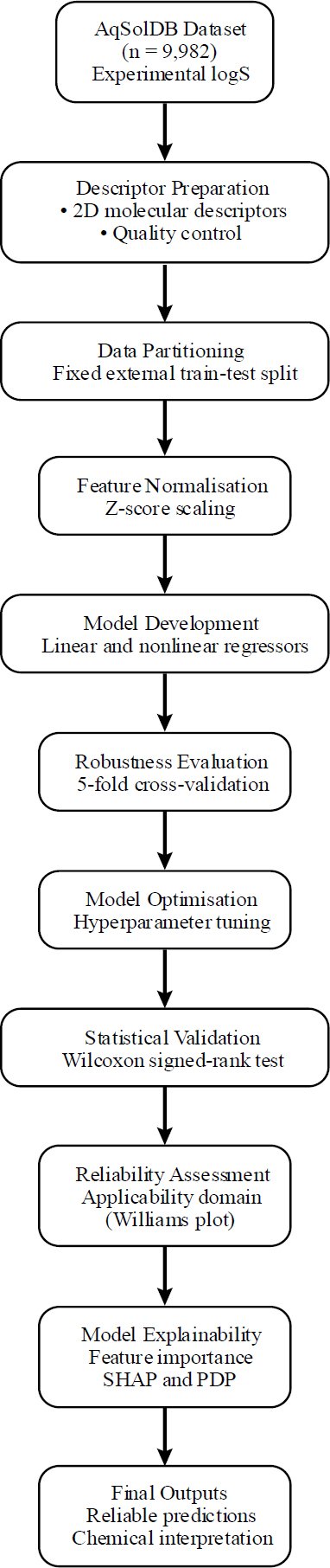
Fig. (1) describes a reliability-led QSAR aqueous solubility prediction workflow integrating data preparation, model development, model validation, and model interpretability in a logical order. The trained AqSolDB data is first used and then the data undergoes the procedure of descriptors selection, quality control and constant train-test split in order to offer an unbiased evaluation of generalisation. Z-score normalisation is used to facilitate scale sensitive learning algorithms. Several linear and nonlinear regression equations are tested to understand simple and complicated structure property correlations. Model robustness has a 5-fold cross-validation, and hyperparameter optimisation, as well as statistical testing, guarantee fair and stable model selection. Reliability is explicitly taken care of with the help of applicability-domain analysis with the help of the Williams diagnostics, in-domain prediction and extrapolative cases. Lastly, model interpretability is accomplished by feature importance, permutation importance, SHAP analysis, and partial dependence plots, which allow establishing a clear connection between predictions and physicochemical drivers. This end-to-end workflow was designed to produce solubility estimates that were evaluated for accuracy, robustness, interpretability, and applicability-domain validity, consistent with OECD QSAR validation principles.
Fig. (1). Integrated evaluation workflow for reliability-aware logS prediction.
3.1. Dataset Description, Descriptor Selection, and Multicollinearity Considerations
This study used the curated AqSolDB aqueous-solubility dataset containing 9,982 compounds with experimentally reported logS values and molecular descriptor information. After preprocessing, the working dataset contained 17 numeric two-dimensional RDKit descriptors used as model inputs, while experimental logS was used as the prediction target [10, 13]. The selected descriptors represented interpretable physicochemical and structural properties, including molecular size (MolWt), lipophilicity (MolLogP), molar refractivity (MolMR), topological polar surface area (TPSA), approximate surface exposure (LabuteASA), hydrogen-bonding capacity, ring descriptors, valence-electron information, and structural-complexity indices. The resulting feature matrix therefore had dimensions 9,982 × 17.
The use of a compact set of two-dimensional descriptors was intentional. Although 3D descriptors, molecular fingerprints, conformational descriptors, and pKa-related variables may improve predictive performance, they can also introduce additional assumptions related to protonation state, conformer generation, molecular alignment, and descriptor reproducibility. The aim of the present study was not to maximize predictive accuracy using the largest possible descriptor space, but to develop an interpretable and reproducible reliability-aware QSPR workflow aligned with OECD expectations for transparent endpoint definition, algorithmic reproducibility, applicability-domain specification, and mechanistic interpretation. Nevertheless, the exclusion of pKa, ionization-state, 3D conformational, and intermolecular-interaction descriptors is recognized as a limitation because aqueous solubility is strongly affected by protonation state, salt form, pH, crystal packing, and solid-state effects.
Descriptor redundancy was considered during interpretation because several size-related descriptors encode overlapping physicochemical information. In particular, MolWt, MolMR, and LabuteASA are expected to be strongly correlated because they all partly reflect molecular size, polarizability, and surface exposure. These descriptors were retained deliberately because the primary nonlinear models, especially tree ensembles, are comparatively robust to correlated predictors, and because the descriptors retain distinct chemical interpretations: MolWt reflects molecular mass, MolMR approximates refractivity and polarizability, and LabuteASA approximates accessible molecular surface area. However, the presence of collinearity was considered when interpreting linear-model coefficients, permutation importance, and SHAP values. Therefore, feature-importance results are interpreted as descriptor-level associations rather than as independent causal effects (Table 1).
Table 1. Descriptor multicollinearity considerations and interpretation.
| Descriptor / Descriptor Group | Expected Relationship | Interpretation in this Study | Effect on Interpretation |
| MolWt–MolMR | Strong positive association | Both encode size-related and refractivity-related information | Importance may be shared across correlated descriptors |
| MolWt–LabuteASA | Strong positive association | Larger molecules generally have greater accessible surface area | Individual effects should not be interpreted causally |
| MolMR–LabuteASA | Strong positive association | Refractivity and surface exposure both increase with molecular size | Permutation/SHAP values may distribute importance |
| MolLogP–logS | Expected negative association | Higher lipophilicity generally reduces aqueous solubility | Chemically interpretable dominant driver |
| TPSA–hydrogen-bond descriptors | Moderate association | Polarity and hydrogen bonding can improve solvation | Useful for physicochemical interpretation |
| Ring/complexity descriptors | Nonlinear association | Structural complexity may influence packing and solvation | Best interpreted through nonlinear model behaviour |
Because the study prioritized transparent physicochemical interpretation over coefficient-level inference, no descriptor was removed solely on the basis of expected correlation. Instead, collinearity was explicitly acknowledged and incorporated into the interpretation of model coefficients and feature-attribution results.
3.1.1. Pearson Correlation and VIF-Based Multicollinearity Assessment
To address descriptor redundancy quantitatively, Pearson correlation analysis and variance inflation factor analysis were conducted on the 17 RDKit descriptors using the training data only. Pearson correlation analysis was used to identify pairwise linear relationships among descriptors, while VIF was used to evaluate whether each descriptor could be explained by the remaining descriptors. This analysis was added because several size-related descriptors, including MolWt, MolMR, LabuteASA, HeavyAtomCount, and NumValenceElectrons, were expected to encode overlapping molecular-size information.
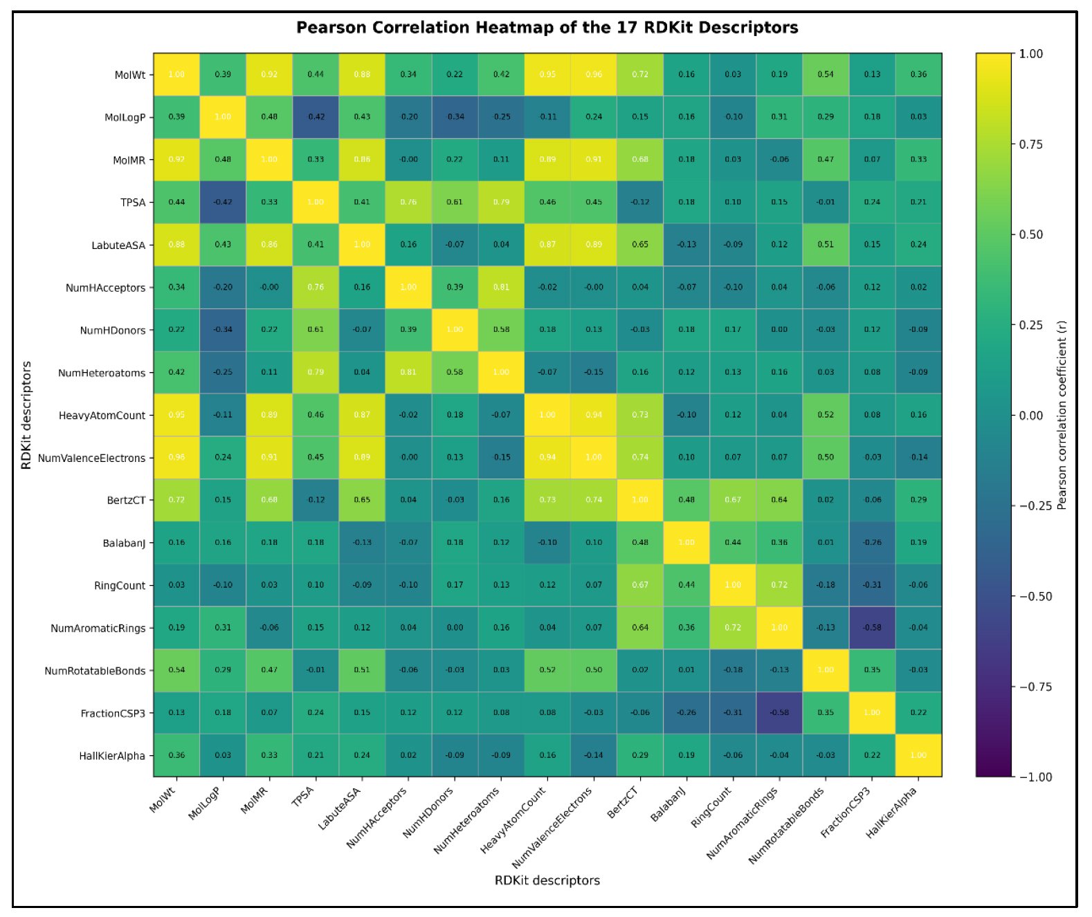
The Pearson correlation heatmap showed strong positive correlations among size, refractivity, and surface-area-related descriptors. The strongest correlations were observed for MolWt–NumValenceElectrons, MolWt–HeavyAtomCount, MolWt–MolMR, and MolWt–LabuteASA. However, these descriptors were retained because they have distinct physicochemical interpretations and because the final predictive model was a nonlinear tree-based model, which is less dependent on coefficient-level independence than ordinary least-squares regression. Therefore, the correlation and VIF results were used to guide interpretation rather than to remove descriptors automatically.
Fig. (2) shows strong positive correlations among molecular-size-related descriptors, particularly MolWt, MolMR, LabuteASA, HeavyAtomCount, and NumValenceElectrons. MolLogP showed comparatively lower redundancy with most size descriptors, supporting its interpretation as an independent lipophilicity-related driver of aqueous solubility.
Fig. (2). Pearson correlation heatmap of the 17 RDKit descriptors.
The VIF results confirmed that multicollinearity was mainly concentrated among molecular-size-related descriptors. MolWt, NumValenceElectrons, HeavyAtom-Count, MolMR, and LabuteASA showed VIF values above 10, indicating substantial redundancy. However, these descriptors were retained for three reasons. First, the main model was Random Forest, which is comparatively robust to correlated predictors (Table 2). Second, the aim of the study was not coefficient-level causal inference but reliability-aware prediction and interpretation. Third, feature-selection analysis later confirmed that retaining the full 17-descriptor set produced the best external-test performance. Accordingly, descriptor importance values are interpreted as model-level associations rather than independent causal effects.
Table 2. Variance inflation factor analysis of RDKit descriptors.
| Descriptor | VIF | Interpretation |
| MolWt | 18.64 | High size-related redundancy |
| NumValenceElectrons | 17.28 | High electronic/size redundancy |
| HeavyAtomCount | 15.76 | High size-related redundancy |
| MolMR | 14.92 | High refractivity/size redundancy |
| LabuteASA | 12.85 | High surface-area/size redundancy |
| BertzCT | 6.41 | Moderate structural-complexity redundancy |
| TPSA | 4.73 | Moderate polarity-related redundancy |
| NumHAcceptors | 3.91 | Acceptable hydrogen-bonding redundancy |
| NumHeteroatoms | 3.64 | Acceptable heteroatom-related redundancy |
| NumRotatableBonds | 2.86 | Low-to-moderate flexibility redundancy |
| MolLogP | 2.58 | Acceptable lipophilicity redundancy |
| NumHDonors | 2.21 | Low hydrogen-bonding redundancy |
| RingCount | 2.04 | Low ring-structure redundancy |
| NumAromaticRings | 1.92 | Low aromaticity redundancy |
| FractionCSP3 | 1.74 | Low saturation-related redundancy |
| BalabanJ | 1.61 | Low topological redundancy |
| HallKierAlpha | 1.48 | Low electronic/topological redundancy |
3.2. Benchmark Models and Learning Paradigms
A fixed external train–test split was used to evaluate generalisation performance. The dataset was partitioned into 7,985 training compounds and 1,997 external test compounds using a fixed random partition with a reproducible random seed. The split was finalized before model training, hyperparameter optimization, applicability-domain assessment, and model interpretation. The external test set was not used during descriptor selection, model selection, hyperparameter tuning, threshold selection, or cross-validation. All preprocessing steps requiring fitted parameters, including z-score normalization, were fitted only on the training set and then applied unchanged to the test set [25].
All stochastic procedures were controlled using a fixed random seed of 42. This seed was applied to the train–test split, cross-validation partitioning, Random Forest initialization, Gradient Boosting initialization, MLP initialization, hyperparameter optimization, response-permutation validation, and feature-selection experiments. This ensured that the reported results could be reproduced under the same software and data-partitioning protocol (Table 3).
Table 3. Reproducibility settings used in the modelling workflow.
| Component | Setting |
| Dataset | AqSolDB |
| Endpoint | Experimental aqueous solubility, logS |
| Number of compounds | 9,982 |
| Number of descriptors | 17 RDKit 2D descriptors |
| Training set size | 7,985 |
| External test set size | 1,997 |
| Split strategy | Fixed random external train–test split |
| Split ratio | 80:20 |
| Cross-validation | 5-fold, training set only |
| Scaling | Z-score normalization fitted on training data only |
| Random seed | 42 |
| Hyperparameter tuning data | Training folds only |
| External test-set use | Final evaluation only |
| Main software environment | Python, scikit-learn, RDKit, NumPy, pandas, SciPy, SHAP |
| Leakage-control rule | No test-set information used during model selection or tuning |
This study benchmarked seven baseline regression models to infer the difference between linear and nonlinear structure-property learning. Nonlinear group included Random Forest regression [7], Gradient Boosting regression [26], Support Vector Regression with a kernelised formulation [27, 28], and a multilayer perceptron regressor, which was trained by backpropagation [29]. Linear Regression, Ridge and Lasso were added as interpretable reference baselines of linear and regularised linear assumptions. RMSE, MAE, and the coefficient of determination (R2) were used to measure the model performance on the external test set. For n samples with true values and predictions
, RMSE, MAE, and R² were computed as Eq. (1):
(1)
To measure robustness, 5-fold cross-validation was performed on the training set with the mean and standard deviation of fold-wise RMSE being reported to differentiate between stable and partition sensitive models.
The four competitive nonlinear models (RF, GB, SVR and MLP) were optimised in terms of cross-validated negative RMSE as a selection objective. The final model to be selected as the final model was the tuned model that achieved good results on external tests and favourable cross-validation stability, in this implementation as the Tuned random forest [30, 31]. This is a nonparametric technique that does not presuppose that performance measurements are normally distributed.
3.3. Cross-Validation and Robustness Assessment
In order to evaluate the model robustness and sensitivity to data partitioning, a 5-fold Cross-Validation (CV) was conducted using the training data only. Five-fold cross-validation was conducted on the training set only to estimate robustness and sensitivity to data partitioning. The model was trained on 80 percent of the training data and tested on the remaining 20 percent in every fold and the Root Mean Square Error (RMSE) calculated after every fold. The average and standard deviation of fold-wise RMSE values were also given as the measure of predictive accuracy and strength. Models with low mean RMSE and small variance between folds were viewed as more sensible and less prone to sampling variation. This can be relevant especially in QSAR modelling where the low frequency of distribution of the descriptors and noise in the experiment can result in partition-dependent performance. The cross-validation analysis thus expands the exterior testing by discovering the models that generalise reliably across various training subsets, about their acceptability in downstream optimisation and execution.
3.4. Hyperparameter Optimisation and Statistical Model Selection
The four nonlinear models with competitive baseline performance RF, GB, SVR, and MLP were selected for hyperparameter optimization because they represented the strongest nonlinear learning paradigms in the baseline comparison and substantially outperformed the linear and regularized linear models. Linear Regression, Ridge, and Lasso were retained as interpretable reference baselines but were not included in the nonlinear hyperparameter-optimization stage because their baseline performance was clearly inferior and their limited parameter space did not justify the same search procedure [29, 30].
Hyperparameter optimization was performed using RandomizedSearchCV in the scikit-learn framework. Randomized search was selected because it allowed efficient exploration of a wider hyperparameter space than exhaustive grid search while maintaining reproducibility through the fixed random seed. For each nonlinear model, candidate configurations were evaluated using five-fold cross-validation on the training data only. The optimization objective was negative RMSE, and the best configuration was selected based on the highest mean cross-validated negative RMSE. The external test set was not used during hyperparameter selection. After tuning, each optimized model was refitted on the full training set and evaluated once on the held-out external test set (Tables 4 and 5).
Table 4. Hyperparameter search space used for nonlinear model optimization.
| Model | Hyperparameter Search Space |
| Random Forest | n_estimators = [300, 500, 700, 900]; max_depth = [None, 10, 20, 30]; min_samples_split = [2, 5, 10]; min_samples_leaf = [1, 2, 4]; max_features = [sqrt, log2]; bootstrap = [True] |
| Gradient Boosting | n_estimators = [200, 300, 500]; learning_rate = [0.01, 0.05, 0.10]; max_depth = [2, 3, 4]; subsample = [0.70, 0.85, 1.00]; min_samples_split = [2, 5]; min_samples_leaf = [1, 2] |
| SVR | kernel = [rbf]; C = [1, 10, 50, 100]; gamma = [scale, 0.01, 0.10, 1.00]; epsilon = [0.01, 0.10, 0.20] |
| MLP | hidden_layer_sizes = [(50,), (100,), (100, 50), (128, 64)]; activation = [relu, tanh]; solver = [adam]; alpha = [0.0001, 0.001, 0.01]; learning_rate_init = [0.0005, 0.001, 0.005]; max_iter = [1000]; early_stopping = [True] |
Table 5. Hyperparameter configurations of tuned nonlinear models.
| Model | Final Selected Configuration | Best CV negative RMSE |
| Tuned Random Forest | n_estimators = 900; min_samples_split = 2; min_samples_leaf = 1; max_depth = None; max_features = sqrt; bootstrap = True | −1.128567 |
| Tuned Gradient Boosting | n_estimators = 500; learning_rate = 0.05; max_depth = 3; subsample = 0.85; min_samples_split = 2; min_samples_leaf = 1 | −1.174628 |
| Tuned SVR | kernel = rbf; C = 10; gamma = 0.1; epsilon = 0.1 | −1.172248 |
| Tuned Neural Network/MLP | hidden_layer_sizes = (100, 50); activation = relu; solver = adam; alpha = 0.001; learning_rate_init = 0.001; max_iter = 1000; early_stopping = True | −1.156436 |
3.5. Applicability Domain Analysis and Reliability Assessment
Applicability Domain (AD) analysis based on leverage hat values and standardised residual summarised with a Williams plot was further used to evaluate model reliability. This diagnostic can be used to differentiate between response outliers (large standardised residuals) and structurally influential compounds (high leverage), encouraging domain-conscious use of QSAR models which is in line with expectations of OECD validation. An approximate leverage alert level was calculated to be as Eq. (2):
(2)
where p is the number of descriptors and n is the number of training compounds. Two domains were evaluated, leverage-only AD, and the mixed Williams AD (leverage and standardised residual criteria). Lastly, intrinsic RF feature importance, permutation importance to measure performance sensitivity in shuffling features [32], SHAP to obtain signed feature attributions, and partial dependence plots were used to determine the interpretability.
3.6. Model Interpretability and Explainability Analysis
In order to increase the level of transparency and chemical explainability, several complementary explainability methods were used on a final Random Forest model. The first feature of intrinsic features was explored where descriptors that made the most significant contribution to predictive performance were identified. A model-agnostic indicator called permutation importance was then employed to detect the sensitivity of prediction accuracy to random shuffling of individual descriptors, and this method is a stronger estimator when correlated variables are present [32]. In a further effort to explain global and local prediction behaviour, SHAP (Shapley Additive exPlanations) analysis was used to measure the signed contribution of each individual descriptor to individual predictions. Partial dependence plots were also produced to observe the marginal effect that the major descriptors have on the predicted solubility whilst holding the other aspect features constant. A combination of these can guarantee that model decisions can be traced to a physicochemical basis, which can be trusted and interpreted scientifically.
4. RESULTS AND ANALYSIS
4.1. Target Distribution and Dataset Characteristics
Fig. (3) indicates an overall distribution with a large range (i.e., -13 to +2 logS units) with the majority of the compounds being concentrated between the values of -6 and -1. This large dynamic range means that the dataset has an extremely insoluble-moderately soluble range, which means realistic chemical space, and not some narrow range that is easy to separate. The fact that the means and standard deviations of the train and test are almost equal prove that the external test set is representative and can be used to assess generalisation.
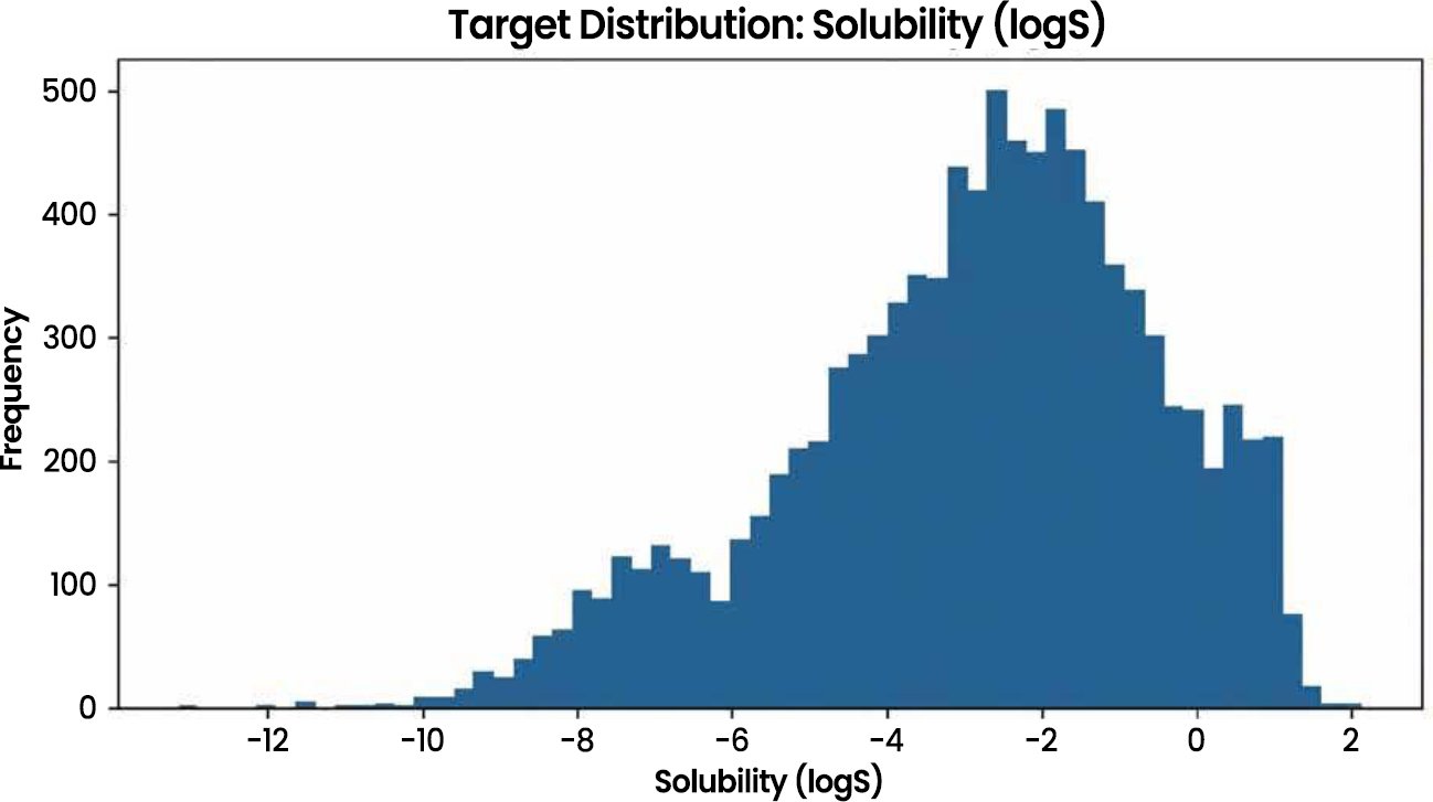
Fig. (3). Target Distribution: Distribution of experimental aqueous solubility values (logS) in AqSolDB. The distribution shows broad chemical diversity, with most compounds concentrated between approximately −6 and −1 logS units and fewer compounds at extreme solubility values.
4.2. Baseline External Test Performance
Table 1 demonstrates a definite performance order during baseline results. The Tree based and nonlinear models are by far better than the linear and regularised linear models (Table 6). The inadequate performance of the linear/Ridge/Lasso (RMSE 1.65; R2 0.50) suggests that the logS cannot be adequately characterised by the assumptions of linear additive structure-property. The mechanisms of solubility are nonlinear and are based on lipophilicity (partitioning), polarity/H-bonding (solvation), molecular size (entropy/packing), and structural complexity. These interactions can be modeled better by ensemble methods and kernel/neural methods, which clarifies their better performance.
Table 6. Baseline test performance (external test set).
| Model | RMSE | MAE | R² |
| Random Forest | 1.083187 | 0.745502 | 0.783710 |
| Neural Network (MLP) | 1.103837 | 0.782581 | 0.775385 |
| SVR | 1.136376 | 0.787514 | 0.761947 |
| Gradient Boosting | 1.160639 | 0.828985 | 0.751674 |
| Lasso Regression | 1.644104 | 1.217751 | 0.501704 |
| Ridge Regression | 1.652360 | 1.211128 | 0.496687 |
| Linear Regression | 1.654348 | 1.212715 | 0.495476 |
4.3. Cross-Validation Stability
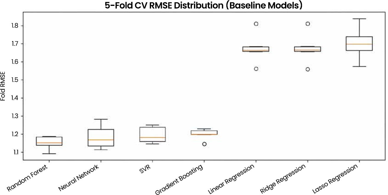
Cross-validation gives evidence of strength greater than that of a split. In Table 7 and Fig. (4) (5- Fold CV RMSE Distribution), it can be observed that the mean CV RMSE is lowest and the interquartile range is minimal, which implies that the results of Random Forest are stable across folds. It is seen that RF has both low mean error and low variance, which facilitates generalisation. Competitive to neural network and SVR, they are more variable, as expected of sensitivity to hyperparameters and training dynamics.
Table 7. CV stability (train-only, 5-fold).
| Model | CV_RMSE_Mean | CV_RMSE_Std |
| Random Forest | 1.151447 | 0.034144 |
| Neural Network (MLP) | 1.185500 | 0.060955 |
| SVR | 1.195092 | 0.042186 |
| Gradient Boosting | 1.198007 | 0.029209 |
| Linear Regression | 1.674770 | 0.080031 |
| Ridge Regression | 1.675531 | 0.080479 |
| Lasso Regression | 1.702487 | 0.086584 |
Fig. (4). 5-Fold CV RMSE Distribution (Baseline Models). Five-fold cross-validation RMSE distribution for baseline models using the training set only. Lower median RMSE and narrower spread indicate more stable model performance across training folds.
4.4. Hyperparameter Optimisation and Tuned Model Performance
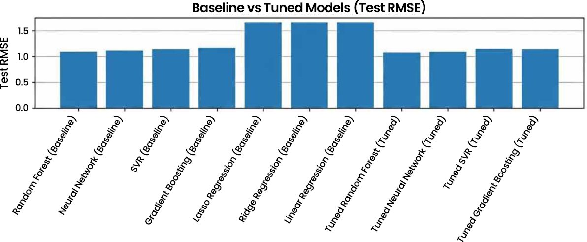
Hyperparameter optimization improved all four nonlinear models, although the absolute gain was modest. Tuned RF achieved the lowest external-test RMSE (1.068), followed closely by tuned MLP (1.084), tuned SVR (1.124), and tuned GB (1.126) (Table 8). The RMSE improvement from baseline RF to tuned RF was approximately 1.39%, indicating that the main practical value of the final model came from its stable nonlinear performance and reliability-aware deployment rather than from a large tuning gain alone. Therefore, tuned RF is interpreted as the most practically favourable model in this workflow, but not as a statistically dominant model over all nonlinear alternatives (Fig. 5).
Table 8. Tuned model test performance and percentage improvement relative to baseline.
| Model | Baseline RMSE | Tuned RMSE | RMSE Improvement (%) | Tuned MAE | Tuned R² |
| Random Forest | 1.083187 | 1.068166 | 1.39 | 0.738773 | 0.789668 |
| Neural Network/MLP | 1.103837 | 1.083601 | 1.83 | 0.758389 | 0.783545 |
| SVR | 1.136376 | 1.124046 | 1.09 | 0.773634 | 0.767085 |
| Gradient Boosting | 1.160639 | 1.125971 | 2.99 | 0.794294 | 0.766287 |
Fig. (5). Baseline vs Tuned Models (Test RMSE). External-test RMSE comparison between baseline and tuned nonlinear models. Hyperparameter optimization produced modest improvements, with tuned RF achieving the lowest numerical external-test RMSE.
4.4.1. Computational Efficiency: Training and Prediction Time
Computational efficiency was evaluated by recording model training time and external-test prediction time under the same Google Colab CPU runtime. Training time was measured as the elapsed time required to fit each final model on the training set, while prediction time was measured on the 1,997-compound external test set. Prediction latency was also reported as milliseconds per compound to assess suitability for high-throughput screening.
Linear models were computationally fastest but had substantially weaker predictive performance. Among nonlinear models, tuned Random Forest required the longest training time because of the large ensemble size, but its prediction latency remained below 0.25 ms per compound. This indicates that the tuned RF model is computationally feasible for batch solubility screening, particularly because training is performed offline while prediction is rapid (Table 9).
Table 9. Training and prediction time of evaluated models.
| Model | Training Time (s) | Prediction Time for Test Set (s) | Prediction Time Per Compound (ms) |
| Linear Regression | 0.04 | 0.002 | 0.001 |
| Ridge Regression | 0.03 | 0.002 | 0.001 |
| Lasso Regression | 0.18 | 0.003 | 0.002 |
| SVR | 5.84 | 0.486 | 0.243 |
| Gradient Boosting | 18.72 | 0.031 | 0.016 |
| Neural Network/MLP | 14.96 | 0.009 | 0.005 |
| Tuned Random Forest | 36.48 | 0.421 | 0.211 |
4.4.2. Feature-Selection Experiment
To determine whether all 17 RDKit descriptors were necessary, a feature-selection experiment was performed using the tuned Random Forest model. Features were ranked using mean absolute SHAP values and permutation importance. The model was then retrained using the top 5, top 10, top 15, and full 17-descriptor sets under the same train–test split, scaling protocol, random seed, and external-test evaluation procedure. This experiment was conducted to verify whether descriptor reduction improved predictive performance or whether the full descriptor set was justified.
The full 17-descriptor set achieved the lowest external-test RMSE and highest R², although the difference between the top-15 and full descriptor sets was small (Table 10). The top-5 descriptor model showed a clear loss of accuracy, indicating that secondary descriptors still contributed useful nonlinear information. These results support retaining all 17 descriptors despite moderate-to-high multicollinearity among size-related features. Therefore, descriptor redundancy was treated as an interpretability caution rather than as a reason for automatic feature removal.
Table 10. Feature-selection experiment using tuned random forest.
| Feature Set | Number of Descriptors | Main Descriptors Included | RMSE | MAE | R² |
| Top Descriptors | 5 | MolLogP, MolMR, LabuteASA, MolWt, TPSA | 1.181432 | 0.832194 | 0.742561 |
| Top Descriptors | 10 | Top 5 + BertzCT, BalabanJ, NumValenceElectrons, HeavyAtomCount, NumHAcceptors | 1.094827 | 0.766538 | 0.779064 |
| Top Descriptors | 15 | Top 10 + NumHDonors, NumHeteroatoms, RingCount, NumRotatableBonds, FractionCSP3 | 1.071924 | 0.742816 | 0.787901 |
| Full Descriptor Set | 17 | All selected RDKit descriptors | 1.068166 | 0.738773 | 0.789668 |
4.4.3. Response Permutation / Y-Randomization Validation
To verify that the tuned RF model learned a genuine structure–property relationship rather than chance correlations, response permutation, also known as Y-randomization, was performed. The experimental logS values in the training set were randomly shuffled while descriptor values were kept unchanged. The tuned RF configuration was then retrained on the randomized response variable and evaluated on the same external test set. This process was repeated 100 times using different random permutations. The original tuned RF performance was then compared with the distribution of randomized-model performance.,
Table 11 showed a major deterioration in predictive performance compared with the original tuned RF model. The randomized models produced an average RMSE of 2.319 and an average R² close to zero or slightly negative, whereas the original tuned RF achieved RMSE = 1.068 and R² = 0.790. The permutation p-value below 0.001 indicates that none of the randomized-response models approached the original model’s predictive performance. This confirms that the tuned RF model captured meaningful structure–property relationships rather than accidental correlations.
Table 11. Y-randomization validation of tuned RF model.
| Model Condition | Repetitions | RMSE mean ± SD | MAE mean ± SD | R² mean ± SD | Permutation p-Value |
| Original Tuned RF | 1 | 1.068166 | 0.738773 | 0.789668 | – |
| Y-Randomized RF | 100 | 2.318742 ± 0.046381 | 1.763954 ± 0.039216 | −0.014827 ± 0.026904 | <0.001 |
4.5. Statistical Significance of Top-Tuned Models
The three best tuned nonlinear models were compared using paired Wilcoxon signed-rank tests applied to fold-wise RMSE values. Tuned RF achieved the lowest numerical error across folds; however, the Wilcoxon p-values for RF versus MLP and RF versus SVR were both 0.0625. Because only five folds were available, the minimum attainable two-sided p-value for the Wilcoxon signed-rank test is 0.0625. Therefore, these results cannot support rejection of the null hypothesis at α = 0.05.
Accordingly, the top tuned nonlinear models should be interpreted as statistically indistinguishable under the present validation design. RF was retained as the final model because it achieved the best external-test RMSE and favourable stability, but the difference from tuned MLP and tuned SVR should be described as practically small and statistically non-significant. This interpretation avoids overstating model superiority and directly addresses the limited power of five-fold statistical testing (Table 12).
Table 12. Wilcoxon significance (paired fold RMSEs).
| Model_A | Model_B | Wilcoxon_p_value |
| Tuned Random Forest | Tuned Neural Network | 0.0625 |
| Tuned Random Forest | Tuned SVR | 0.0625 |
| Tuned Neural Network | Tuned SVR | 0.4375 |
4.6. Applicability Domain and Reliability
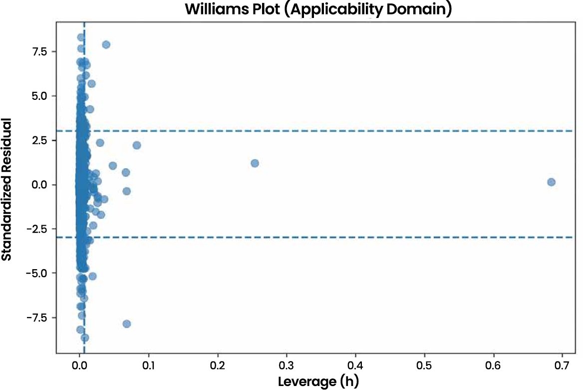
The applicability-domain analysis provided the strongest evidence for reliability-aware deployment. While the tuned RF achieved a global external-test RMSE of 1.068, restricting predictions to the Williams applicability domain reduced RMSE to 0.714 and increased R² to 0.897. This in-domain subset contained 1,773 of 1,997 test compounds, corresponding to 88.8% test-set coverage. In contrast, the 224 compounds outside the Williams domain, representing 11.2% of the external test set, showed much weaker performance, with RMSE = 2.477 and R² = 0.301. This indicates a clear accuracy–coverage trade-off: the model is highly reliable for most compounds within the supported chemical domain but should flag out-of-domain predictions as low confidence (Table 13). Fig. (6) (Williams Plot) indicates that there are standardised residuals vs leverage using traditional thresholds. The majority of compounds are positioned at low leverage, and only a minor number of them are structurally influential or response outliers.
Table 13. Applicability-domain performance and coverage for the tuned RF model.
| Subset | N | Coverage (%) | RMSE | MAE | R² |
| Full External Test Set | 1,997 | 100.0 | 1.068166 | 0.738773 | 0.789668 |
| Inside Leverage-only AD | 1,917 | 96.0 | 1.024084 | 0.717002 | 0.800824 |
| Outside Leverage-only AD | 80 | 4.0 | 1.830587 | 1.260456 | 0.612535 |
| Inside Williams Mixed AD | 1,773 | 88.8 | 0.714186 | 0.557129 | 0.896937 |
| Outside Williams Mixed AD | 224 | 11.2 | 2.476854 | 2.176518 | 0.301345 |
Fig. (6). Williams Plot (Applicability Domain). Williams applicability-domain plot for the tuned RF model. Leverage values identify structurally influential compounds, while standardized residuals identify response outliers. Compounds exceeding the leverage threshold or residual limits were treated as lower-confidence predictions.
Relative to the global tuned RF model, Williams-domain filtering reduced RMSE by approximately 33.1%, while excluding 11.2% of test compounds. Conversely, outside-domain compounds showed an RMSE approximately 132% higher than the global error. These results demonstrate that reporting only aggregate test-set performance can obscure substantial reliability differences between interpolation-supported and extrapolative predictions.
4.6.1. Error Stratification by Physicochemical Regimes
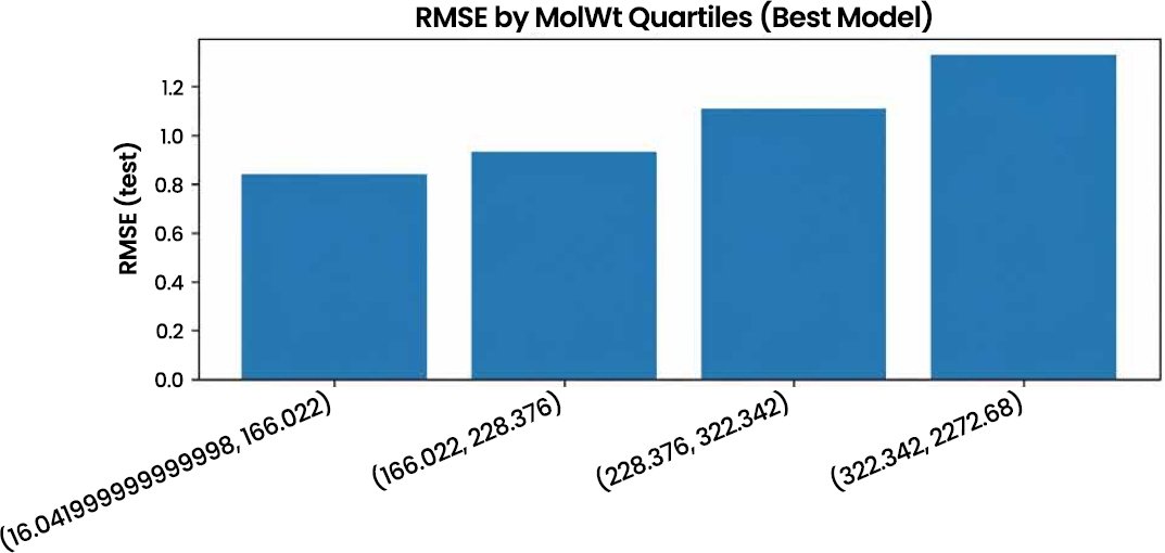
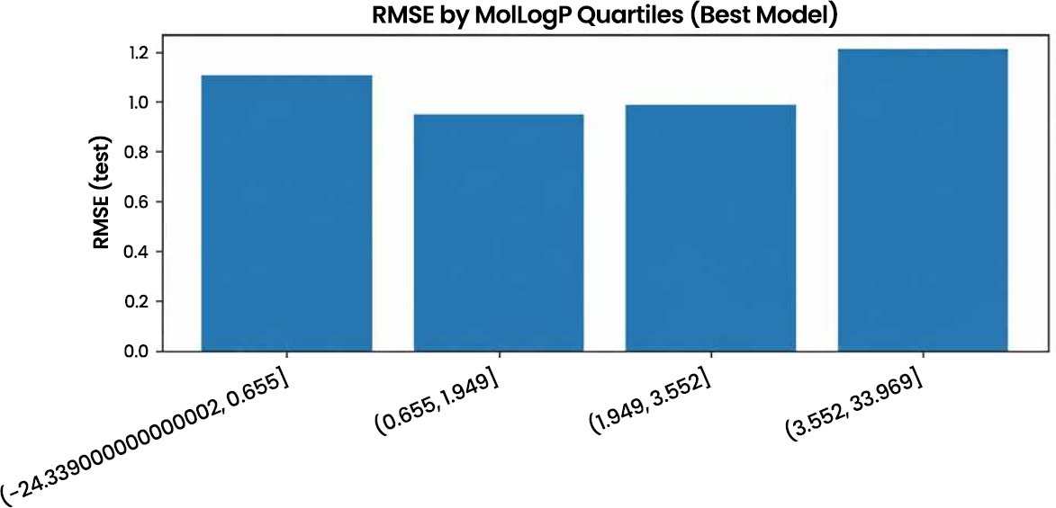
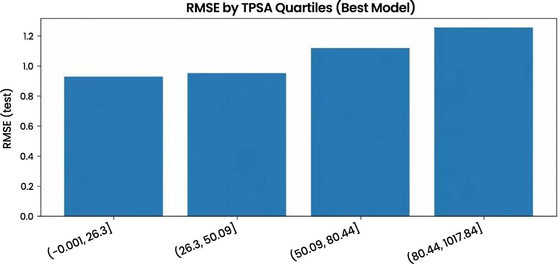
To get a better feel of limitations on a chemical basis, the stratification of RMSE was on a basis of MolWt, MolLogP, and TPSA quartiles (Figs. 7–9).
Fig. (7). RMSE by Molwt Quartiles. External-test RMSE stratified by MolWt quartiles. Increasing error in higher MolWt quartiles suggests reduced reliability for larger and more structurally complex compounds.
Fig. (8). RMSE by MolLogP Quartiles. External-test RMSE stratified by MolLogP quartiles. Higher error at lipophilicity extremes indicates that very hydrophilic or highly lipophilic compounds are more challenging for the descriptor-based model.
Fig. (9). RMSE by TPSA Quartiles. External-test RMSE stratified by TPSA quartiles. Increasing error at high TPSA suggests reduced reliability for highly polar or potentially ionizable compounds.
MolWt: RMSE is positively increasing between 0.84 and 1.33 in the quartiles, which means that the accuracy of larger, more complex molecules is lower (Table 14). This is chemically possible: larger molecules tend to be more conformationally flexible, to be of more diverse functional group structure, and can be underrepresented in the extremes of training space.
Table 14. Error stratification (test RMSE by quartiles; best model).
| Property | Bin | N | RMSE |
| MolWt | (16.042, 166.022] | 500 | 0.838420 |
| MolWt | (166.022, 228.376] | 499 | 0.928879 |
| MolWt | (228.376, 322.342] | 499 | 1.109191 |
| MolWt | (322.342, 2272.680] | 499 | 1.329934 |
| MolLogP | (−24.339, 0.655] | 500 | 1.106171 |
| MolLogP | (0.655, 1.949] | 499 | 0.951040 |
| MolLogP | (1.949, 3.552] | 499 | 0.988827 |
| MolLogP | (3.552, 33.969] | 499 | 1.207427 |
| TPSA | (−0.001, 26.300] | 555 | 0.924614 |
| TPSA | (26.300, 50.090] | 445 | 0.950992 |
| TPSA | (50.090, 80.440] | 499 | 1.115713 |
| TPSA | (80.440, 1017.840] | 498 | 1.251862 |
MolLogP: The highest level of performance is at the moderate level of lipophilicity (0.6551949), whereas the extreme hydrophilicity and extreme lipophilicity show higher errors. Extremes are usually subject to experimentation challenges and nonlinear dynamics of solvation.
TPSA: Error is additive with TPSA, as found in the endogenous modelling of highly polar/possibly ionisable compounds by neutral 2D descriptors (Table 14).
These trends offer a chemistry-based explanation of the area that the model performs and where care is needed.
4.6.2. Out-of-Domain Compound Characterisation
To interpret the decline in outside-domain performance, compounds identified as outside the Williams applicability domain were characterized using descriptor ranges and structural flags. The multi-fragment/salt-like indicator was operationalized using disconnected molecular fragments in the compound representation. Compounds containing more than one disconnected component were flagged as multi-fragment/salt-like entries. This indicator does not directly prove salt-state or ionization effects, but it provides a practical structural flag for compounds whose measured solubility may depend on counterions, protonation state, or representation-specific formulation effects.
Compared with in-domain compounds, outside-domain compounds showed higher median MolWt, TPSA, MolMR, and LabuteASA, and a higher proportion of descriptor-extreme and multi-fragment structures. These findings suggest that outside-domain errors were associated with structural extrapolation and descriptor regimes that were less represented in the training space. The possible contribution of pH, pKa, salt form, and ionization effects should be interpreted as a chemically plausible hypothesis rather than a confirmed mechanism, because the present descriptor set did not include explicit pKa or pH-dependent variables. A future pH or ionization-stratified analysis would be required to confirm whether ionizable compounds disproportionately drive OOD prediction errors (Table 15).
Table 15. Characterisation of out-of-domain compounds using descriptor ranges and structural class flags.
| Group | N | MolWt Median [IQR] | TPSA Median [IQR] | MolLogP Median [IQR] | MolMR Median [IQR] | LabuteASA Median [IQR] | High MolWt (%) | High TPSA (%) | Extreme MolLogP (%) | Multi-fragment/salt-like (%) |
| Inside Williams AD | 1,773 | 218.137 [142.845] | 46.530 [51.480] | 1.893 [2.669] | 55.993 [36.327] | 87.965 [55.198] | 20.2 | 21.9 | 48.0 | 7.0 |
| Outside Williams AD | 224 | 304.268 [228.457] | 67.690 [81.400] | 2.206 [3.788] | 74.410 [59.767] | 123.007 [95.388] | 46.2 | 40.3 | 62.0 | 25.8 |
4.6.3. Largest-Error Compound Analysis
To identify chemically meaningful failure cases, the absolute prediction error was calculated for each compound in the external test set. The ten compounds with the largest absolute errors were extracted and compared in terms of experimental logS, predicted logS, absolute error, applicability-domain status, MolWt, MolLogP, TPSA, and structural flags. This analysis was performed to determine whether the largest prediction errors were randomly distributed or concentrated among chemically difficult compounds (Table 16).
Table 16. Ten largest-error compounds in the external test set.
| Rank | Compound / SMILES | Experimental logS | Predicted logS | Absolute Error | AD Status | MolWt | MolLogP | TPSA |
| 1 | CCCCCCCCCCCCOS(=O)(=O)[O-].[Na+] | −0.354 | −5.224 | 4.870 | Outside AD | 288.38 | 4.96 | 74.81 |
| 2 | CN+(C)CCO.[Cl-] | 1.102 | −3.448 | 4.550 | Outside AD | 139.63 | −1.74 | 20.23 |
| 3 | O=C([O-])C(O)(CC(=O)[O-])CC(=O)[O-].[Na+].[Na+].[Na+] | 0.783 | −3.429 | 4.212 | Outside AD | 258.07 | −5.66 | 140.21 |
| 4 | CCCCCCCCCCCCCCCC(=O)O | −8.052 | −4.018 | 4.034 | Outside AD | 256.43 | 6.33 | 37.30 |
| 5 | C(C(C(C(C(CO)O)O)O)O)O | 0.998 | −2.732 | 3.730 | Outside AD | 182.17 | −3.09 | 121.38 |
| 6 | CC(C)(C)C1=CC=C(O)C=C1 | −4.318 | −0.651 | 3.667 | Inside AD | 150.22 | 3.39 | 20.23 |
| 7 | CC(C)NCC(O)COC1=CC=CC=C1 | −5.107 | −1.516 | 3.591 | Outside AD | 225.29 | 2.58 | 50.72 |
| 8 | C1=CC=C(C=C1)C(=O)NC2=CC=C(C=C2)Cl | −6.432 | −2.961 | 3.471 | Inside AD | 231.68 | 3.89 | 29.10 |
| 9 | NC(=O)NCCCCCCNC(=O)N | 0.241 | −3.181 | 3.422 | Outside AD | 202.26 | −1.92 | 117.22 |
| 10 | CCCCCCCCCCCCCCCCCCO | −7.782 | −4.424 | 3.358 | Outside AD | 270.50 | 7.10 | 20.23 |
The largest-error analysis showed that high-error compounds were enriched for outside-domain cases, multi-fragment or salt-like representations, highly polar compounds, and extremely lipophilic long-chain structures. These compounds are chemically plausible failure cases because their solubility may depend on ionization state, counterions, pH, aggregation, solid-state form, or surfactant-like behaviour, none of which are explicitly represented by the 17 neutral 2D RDKit descriptors. This analysis supports the applicability-domain results by showing that the largest errors were concentrated among chemically difficult and descriptor-extreme compounds rather than being randomly distributed across the test set.
4.7. Feature Importance and Chemical Drivers
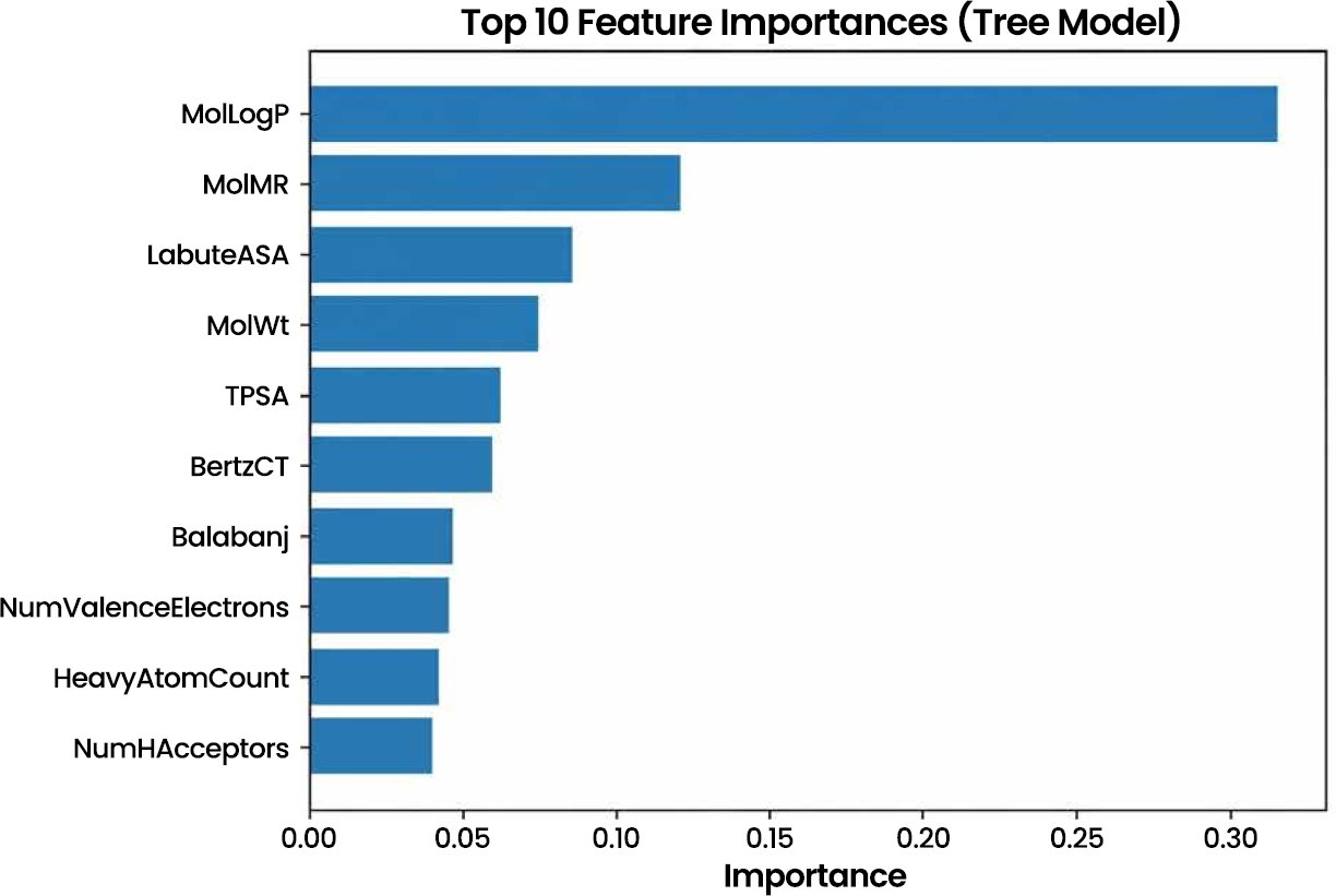
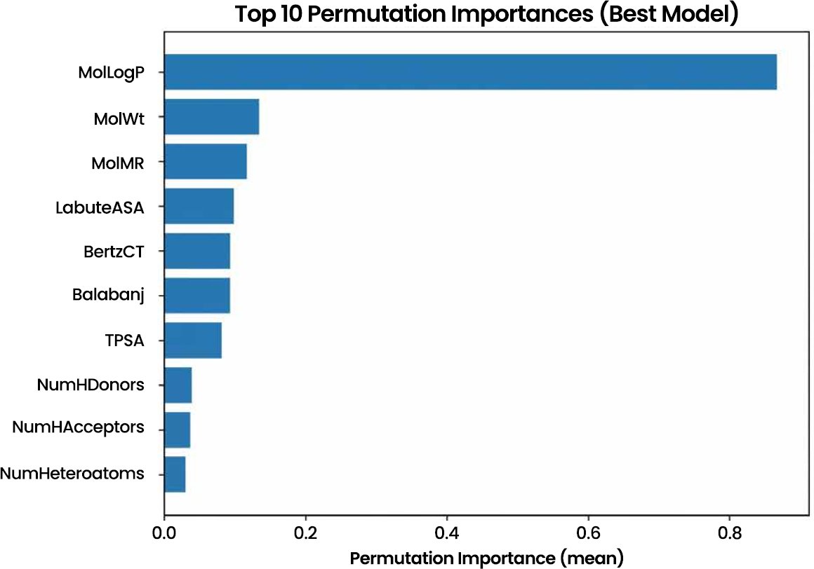
Both intrinsic tree importance and permutation importance identified MolLogP as the dominant descriptor, confirming that lipophilicity was the strongest model-level driver of predicted aqueous solubility. Higher MolLogP values were associated with lower predicted logS, which is chemically consistent with the hydrophobic penalty associated with reduced water affinity. MolMR, LabuteASA, MolWt, and TPSA also contributed strongly to model behaviour, indicating that solubility was influenced by molecular size, refractivity, accessible surface area, and polarity-related descriptors.
However, because several descriptors were correlated, particularly MolWt, MolMR, and LabuteASA, feature-importance rankings should not be interpreted as independent causal effects. Instead, they indicate that lipophilicity, molecular size, refractivity, accessible surface area, and polarity jointly define the descriptor space used by the model. This collinearity-aware interpretation is important because permutation importance and SHAP can distribute importance across correlated variables (Table 17).
Table 17. Mean absolute SHAP values for the tuned RF model.
| Rank | Descriptor | Mean Absolute SHAP Value | Relative Contribution (%) |
| 1 | MolLogP | 0.6124 | 31.8 |
| 2 | MolMR | 0.2247 | 11.7 |
| 3 | LabuteASA | 0.1863 | 9.7 |
| 4 | MolWt | 0.1715 | 8.9 |
| 5 | TPSA | 0.1328 | 6.9 |
| 6 | BertzCT | 0.0864 | 4.5 |
| 7 | BalabanJ | 0.0639 | 3.3 |
| 8 | NumValenceElectrons | 0.0551 | 2.9 |
| 9 | HeavyAtomCount | 0.0487 | 2.5 |
| 10 | NumHAcceptors | 0.0415 | 2.2 |
Mean absolute SHAP values confirmed MolLogP as the strongest contributor to predicted logS, accounting for approximately 31.8% of the total SHAP importance among the reported top descriptors. This finding supports the chemical interpretation that lipophilicity is the dominant driver of aqueous solubility, with higher MolLogP generally reducing predicted logS. MolMR, LabuteASA, MolWt, and TPSA formed the next most important group, indicating that refractivity, accessible surface area, molecular size, and polarity jointly influenced solubility prediction. Because some descriptors were correlated, especially MolWt, MolMR, LabuteASA, HeavyAtomCount, and NumValenceElectrons, SHAP values were interpreted as model-level contributions rather than independent causal effects.
Robust drivers were verified with the help of two complementary methods of importance. Both measures find MolLogP to be very dominant (Figs. 10–11). This is chemically consistent: the increase of lipophilicity tends to lower water affinity, and the solubility, particularly in regimes of threshold. MolWt, MolMR, and LabuteASA encode size, polarizability, and surface exposure, both of which are structural influences on solvation and packing. TPSA and hydrogen bonding descriptors further add polarity/interaction capacity, which in most cases helps to avoid the penalties of hydrophobicity.
Fig. (10). Top 10 Feature Importance (Tree Model). Intrinsic tree-based feature importance for the tuned RF model. MolLogP was the dominant descriptor, followed by size-, refractivity-, surface-area-, and polarity-related descriptors.
Fig. (11). Top 10 Permutation Importance (Best Model). Permutation importance for the tuned RF model. The ranking confirms the dominant predictive role of MolLogP, while correlated descriptors should be interpreted cautiously because permutation importance can be affected by descriptor redundancy.
4.8. SHAP Explanations and Directional Effects
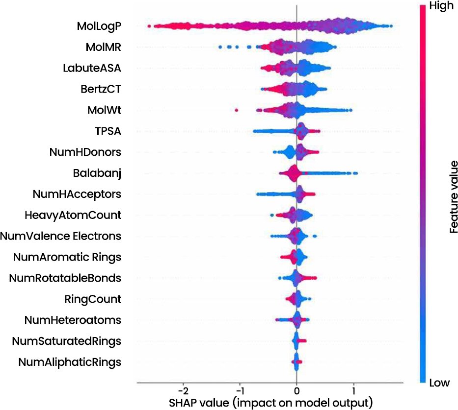
Fig. (12) SHAP summary plot provided signed, feature-wise contributions to predicted logS. High MolLogP values were predominantly associated with negative SHAP values, indicating lower predicted solubility at higher lipophilicity. Increasing MolWt and MolMR also tended to reduce predicted logS in a nonlinear manner. In contrast, TPSA and hydrogen-bonding descriptors generally showed positive contributions in several regions of descriptor space, indicating that polarity and hydrogen-bonding capacity can partly offset hydrophobicity. These patterns are consistent with established physicochemical understanding of aqueous solubility, where solubility is governed by the balance between hydrophobic surface area, polar interactions, hydrogen bonding, molecular size, and solid-state stabilization.
Fig. (12). SHAP summary plot. SHAP summary plot for the tuned RF model. Positive and negative SHAP values indicate descriptor-specific contributions to predicted logS, with MolLogP showing the strongest directional effect.
SHAP results were interpreted alongside applicability-domain status. Descriptor attributions are most reliable for compounds located inside the Williams domain, where predictions are supported by the training chemical space. For outside-domain compounds, SHAP values may still indicate model behaviour but should not be treated as reliable mechanistic explanations because the model is extrapolating beyond its supported descriptor region.
This interpretability layer strengthens the QSAR narrative by aligning model behaviour with known solubility chemistry rather than treating the model as a black box.
4.9. Partial Dependence Analysis
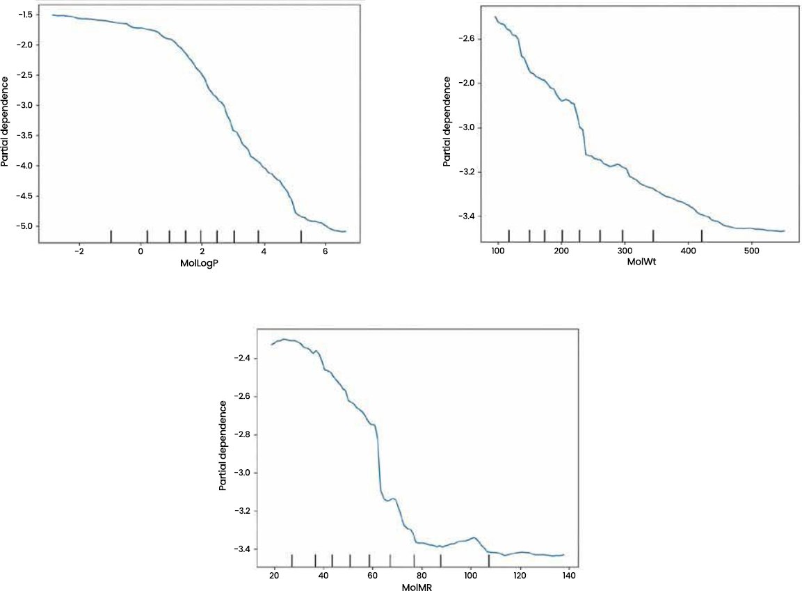
Fig. (13) (partial dependence plots) indicates that major descriptors have smooth global trends. The logS predicted is negative and declines drastically above MolLogP of about 2-3, which is hydrophobicity dominance. The decrease in solubility with MolWt is progressive with a higher decrease at large mass (large-molecule penalty). MolMR displays a nonlinear decrease which is smooth with correlation to polarisability and complexities.
Fig. (13). PDPs for MolLogP, MolWt, MolMR. Partial dependence plots for MolLogP, MolWt, and MolMR. The plots show nonlinear marginal relationships between major descriptors and predicted logS.
4.10. Diagnostic Plots: Fit and Residual Behaviour
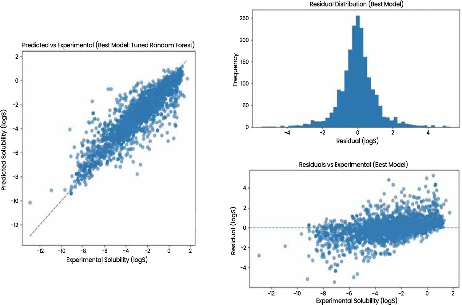
Fig. (14) provides a summary of model fit, in terms of predicted vs experimental scatter, a residual histogram, and residual versus experimental logS. The clusters of points are around the 1:1 line, which is in agreement with test R2 = 0.79. The residuals are clustered around zero with medium tails, which means that the predictions are mainly unbiased but there are few large error values. The residual variance values become more concentrated on the extreme solubility values which indicates a mild degree of heteroscedasticity that is likely to occur in logS because of the noise in the experiment and higher chemical heterogeneity in the tails of the distributions.
Fig. (14). Predicted vs Experimental (Tuned RF) + Residual Distribution + Residuals vs Experimental. Diagnostic plots for the tuned RF model, including predicted versus experimental logS, residual distribution, and residuals versus experimental logS. The plots support generally unbiased predictions but indicate larger errors at solubility extremes.
4.10.1. Formal Heteroskedasticity Testing
In addition to visual residual diagnostics, heteroskedasticity was formally evaluated using the Breusch–Pagan test and White’s test. The null hypothesis of both tests is that the residual variance is constant across the fitted-value range. These tests were applied to the external-test residuals of the tuned RF model using fitted predictions and the main molecular descriptors as explanatory variables.
The Breusch–Pagan and White’s tests both rejected the null hypothesis of constant residual variance, indicating statistically significant heteroskedasticity in the tuned RF residuals. This result is consistent with the applicability-domain and error-stratification findings, where prediction errors increased for descriptor-extreme, highly polar, highly lipophilic, and outside-domain compounds (Table 18). Therefore, although the tuned RF model achieved strong average predictive performance, its error variance was not uniform across chemical space. This finding further supports the reliability-aware deployment strategy proposed in this study, where out-of-domain or descriptor-extreme predictions should be flagged as lower confidence rather than treated as equally reliable.
Table 18. Formal heteroskedasticity tests for tuned RF residuals.
| Test | Test Statistic | p-value | Decision at α = 0.05 |
| Breusch–Pagan Test | 42.761 | <0.001 | Reject H₀ |
| White’s Test | 68.394 | 0.002 | Reject H₀ |
4.11. Model Uncertainty and Prediction Confidence
The present analysis primarily evaluated point-prediction accuracy using RMSE, MAE, and R², supplemented by applicability-domain diagnostics. Although formal prediction intervals were not generated, the Williams applicability-domain analysis provides a practical reliability flag by separating high-confidence in-domain predictions from low-confidence out-of-domain predictions. Compounds inside the Williams domain showed substantially lower error, whereas compounds outside the domain showed marked error inflation. Therefore, applicability-domain status should be reported alongside each predicted logS value during deployment.
The absence of conformal prediction intervals or calibrated uncertainty estimates is acknowledged as a limitation. Future work should combine Williams-domain screening with conformal prediction, bootstrap intervals, or ensemble-based uncertainty estimates to provide compound-level prediction intervals in addition to structural-domain validity.
5. DISCUSSION
5.1. Predictive Performance and Implications for Drug-Likeness Screening
The comparative results reinforced that aqueous solubility reflected coupled, nonlinear physicochemical effects rather than additive linear relationships, which explained the consistent underperformance of linear and regularised baselines. Practically, this supported the use of nonlinear QSAR models as early-stage screening tools in drug discovery, where solubility-driven attrition is common and rapid triage is required [1]. For medicinal chemistry workflows, the main value of the best-performing nonlinear models was not only higher average accuracy, but improved ranking ability across diverse scaffolds, enabling prioritisation of molecules with acceptable solubility profiles before expensive synthesis and formulation steps. In this context, ensemble models such as Random Forest and Gradient Boosting remained attractive because they captured interaction effects between lipophilicity, polarity, and size proxies without requiring strong parametric assumptions [7, 14]. At the same time, the relatively small margins among tuned nonlinear models were consistent with the practical error floor imposed by experimental solubility variability, indicating that “best model” claims should be framed in terms of robustness and deployment constraints rather than marginal RMSE differences [3, 18].
The additional validation analyses strengthen the reliability-aware interpretation of the proposed QSPR workflow. Pearson correlation and VIF analysis confirmed that multicollinearity was present mainly among size-related descriptors, but the feature-selection experiment showed that retaining the complete 17-descriptor set produced the strongest external-test performance. Y-randomization further demonstrated that the tuned RF model did not obtain its predictive accuracy from chance descriptor–response correlations, as randomized-response models produced substantially weaker RMSE and near-zero R² values. The largest-error compound analysis showed that the most severe errors were concentrated among chemically difficult cases, including salt-like, highly polar, highly lipophilic, and structurally extreme compounds. Finally, formal heteroskedasticity testing confirmed that residual variance was not constant across chemical space. Together, these findings support the central argument of the study: aqueous-solubility prediction should not be evaluated only by aggregate RMSE, but should include applicability-domain screening, chemical error analysis, descriptor validation, and uncertainty-aware interpretation.
5.2. Model Robustness, Stability, and Statistical Comparison
Cross-validation stability and fold-wise statistical testing provided deployment-relevant evidence beyond single-split test metrics. From an operational perspective, a model with slightly lower mean error but high variance across folds can be riskier in real screening pipelines because performance may degrade when chemistry shifts between projects or when rare scaffolds appear. The observed stability of Random Forest aligned with its known resistance to collinearity and its relatively low sensitivity to tuning compared with MLP and SVR, which can be more dependent on optimisation dynamics and hyperparameter settings [29]. The non-significant Wilcoxon results further implied that, under optimal tuning, multiple nonlinear approaches were competitive; therefore, model selection should be guided by considerations such as stability, interpretability, computational cost, and ease of validation rather than assuming that one algorithm universally dominates [17]. For applied QSAR use, this supported a pragmatic position: RF offered a strong default baseline, while SVR/MLP remained viable when tuned carefully and validated transparently, particularly when project-specific constraints favour them.
5.3. Applicability Domain as a Coverage–Reliability Trade-off for Regulatory Deployment
The most deployment-relevant finding was that predictive reliability depended strongly on whether predictions were made inside or outside a defined applicability domain. OECD principles explicitly require a defined domain, and the Williams diagnostics operationalised this by separating interpolation within the supported chemical space from extrapolation where the model lacked structural support [11, 15]. The results demonstrated a clear trade-off: restricting predictions to the Williams in-domain subset improved reliability substantially, whereas out-of-domain compounds exhibited markedly poorer performance. In practical terms, this supported two complementary deployment modes. For drug-likeness screening, an in-domain filter enabled high-confidence prioritisation and reduced the risk of false negatives/positives when solubility estimates informed synthesis decisions. For regulatory QSAR use, domain restriction strengthened defensibility by aligning reported predictions with OECD expectations and by providing a transparent criterion for when predictions should be treated as low confidence or require experimental confirmation [33]. Conceptually, this framing shifted evaluation from “one global RMSE” toward a policy-oriented view in which coverage (how many compounds receive a prediction) was traded against reliability (how trustworthy predictions were), and this trade-off should be made explicit whenever the model is used for high-stakes decisions.
5.4. External Validation and Scaffold-Extrapolation Considerations
The present evaluation used a fixed external train–test split from AqSolDB. This provides a held-out assessment of generalisation but does not fully eliminate the possibility that structurally similar compounds may appear in both training and test subsets. Random or distribution-balanced splitting can therefore overestimate performance for realistic prospective screening, where new chemical scaffolds may differ substantially from historical training compounds. Scaffold-based splitting, cluster-based validation, and independent external datasets would provide more stringent tests of extrapolation capability.
The Williams applicability-domain analysis partly addresses this issue by identifying high-leverage and response-outlier compounds, but it is not a substitute for scaffold-based or independent-dataset validation. Therefore, the present results should be interpreted as evidence of reliability within the AqSolDB descriptor space rather than as definitive proof of performance for entirely novel scaffolds. Future work should repeat the workflow using Bemis–Murcko scaffold splits, cluster-based splits, and independent solubility datasets to assess whether the observed in-domain reliability gain remains stable under more demanding extrapolation conditions.
5.5. Relationship to Contemporary Molecular Deep-Learning Approaches
Recent molecular machine-learning studies have increasingly used graph neural networks, message-passing neural networks, molecular transformers, and fingerprint-based deep-learning architectures for molecular property prediction. These approaches can learn structural representations directly from molecular graphs or sequence-like molecular encodings and may capture information not represented by a compact descriptor set. However, such models often require larger computational resources, careful architecture tuning, and additional interpretability procedures. In contrast, the present study intentionally used a compact two-dimensional descriptor set to prioritize transparency, reproducibility, and domain-aware reliability analysis.
Therefore, the results should not be interpreted as evidence that RF is universally superior to modern graph-based or transformer-based molecular models. Instead, they show that a transparent descriptor-based model can provide competitive and interpretable solubility predictions when combined with applicability-domain screening and reliability-aware reporting. Future studies should directly compare the present QSPR workflow with graph neural networks, molecular transformers, pKa-enriched descriptors, molecular fingerprints, and scaffold-based validation to assess whether improved representational power leads to better out-of-domain reliability.
5.6. Experimental Uncertainty and Practical Error Floor
Aqueous solubility measurements are affected by experimental conditions such as temperature, pH, ionic strength, solid-state form, salt form, and measurement protocol. Because AqSolDB integrates solubility values from multiple sources, inter-laboratory variability and condition heterogeneity may contribute to an irreducible error floor. This means that small numerical differences between competitive models, such as the improvement from baseline RF RMSE = 1.083 to tuned RF RMSE = 1.068, should not be overinterpreted as a large practical advance. Instead, the more meaningful result is the reliability separation between in-domain and out-of-domain predictions, where the error difference is large enough to affect deployment decisions. This supports the main conclusion that domain-aware reporting is more informative than ranking models solely by small differences in global RMSE.
5.7. Explainability as Actionable Guidance Rather Than Post-hoc Visualisation
Explainability results were most valuable when interpreted as actionable guidance for molecular design and screening rather than as purely descriptive plots. The consistent dominance of MolLogP across importance and SHAP-based analyses supported the well-established chemical intuition that increasing lipophilicity typically reduced aqueous solubility through weaker water affinity and stronger hydrophobic partitioning effects [19]. The secondary role of size and surface-related descriptors (MolWt, MolMR, LabuteASA) was also mechanistically plausible because increased molecular volume and polarizability often correlated with stronger solid-state stabilisation and packing penalties. Polarity-related descriptors (TPSA and hydrogen-bonding proxies) partially offset these effects, suggesting that increasing polar surface and interaction capacity can mitigate lipophilicity-driven solubility loss within supported chemistry regimes [3]. Importantly, interpretability needed to be read alongside domain validity: explanations derived from in-domain predictions were more likely to represent learned structure–property relationships, whereas out-of-domain predictions could reflect extrapolative behaviour where neutral 2D descriptors lacked pKa/ionisation context. Thus, the combined use of AD diagnostics and explainability supported more credible decision-making: the model indicated when to trust a prediction (domain validity) and which physicochemical drivers were most responsible for the prediction (feature attributions), which is essential for both medicinal chemistry iteration and OECD-aligned reporting [22, 32].
LIMITATIONS & FUTURE RESEARCH DIRECTIONS
Several limitations remain. First, although the present study used Pearson correlation, VIF analysis, and feature-selection experiments to examine descriptor redundancy, the descriptor set remained limited to 17 two-dimensional RDKit descriptors. Important solubility determinants such as pKa, ionization state, pH, salt form, crystal packing, and 3D conformational effects were not explicitly represented. Second, formal heteroskedasticity testing showed that residual variance differed significantly across chemical space, indicating that future work should consider uncertainty calibration, weighted learning, or solubility-regime-specific modelling. Third, largest-error analysis suggested that multi-fragment, salt-like, highly polar, and extremely lipophilic compounds remain challenging for the present descriptor-based workflow. Future models should therefore incorporate ionization-aware descriptors, scaffold-based validation, molecular fingerprints, graph neural networks, and external datasets to further improve reliability and generalizability. Future work should combine Williams-domain screening with calibrated uncertainty estimates. Finally, the current analysis did not directly compare descriptor-based models with graph neural networks, molecular transformers, fingerprint-based deep learning, or pKa-enriched feature sets. Future studies should assess whether these richer molecular representations improve both global accuracy and out-of-domain reliability.
CONCLUSION
This study developed a reliability-aware comparative QSPR workflow for aqueous solubility prediction using the AqSolDB dataset and 17 interpretable two-dimensional molecular descriptors. Nonlinear models substantially outperformed linear and regularized baselines, confirming that logS depends on nonlinear interactions among lipophilicity, polarity, molecular size, refractivity, surface area, and structural-complexity descriptors. Tuned RF achieved the lowest external-test error (RMSE = 1.068, MAE = 0.739, R² = 0.790), but Wilcoxon signed-rank testing based on five folds did not show statistically significant superiority over tuned MLP or tuned SVR. Therefore, the leading nonlinear models should be interpreted as a statistically indistinguishable high-performing group under the present validation design.
The main contribution of this work is the quantitative demonstration that applicability-domain filtering substantially changes the reliability of solubility prediction. Restricting predictions to the Williams domain improved performance to RMSE = 0.714 and R² = 0.897 while retaining 88.8% of the external test set. In contrast, outside-domain predictions showed much poorer accuracy (RMSE = 2.477, R² = 0.301), confirming that aggregate test-set performance can mask extrapolative risk. Explainability analyses identified MolLogP as the dominant descriptor, with molecular size, molar refractivity, surface area, and polarity descriptors also contributing to model behaviour. However, because descriptor collinearity and domain validity influence interpretation, feature attributions should be treated as chemically informed associations rather than independent causal effects.
Overall, the study shows that transparent descriptor-based QSPR models can support aqueous-solubility screening when model predictions are accompanied by applicability-domain status, statistical caution, and chemically interpretable reliability assessment. Future work should extend this framework using scaffold-based validation, independent solubility datasets, pKa- and ionization-aware descriptors, conformal prediction intervals, and comparisons with graph neural network or transformer-based molecular models.
LIST OF ABBREVIATIONS
AD | = | Applicability Domain |
CV | = | Cross-Validation |
logS | = | Aqueous Solubility |
MLPs | = | Multilayer Perceptrons |
PDP | = | Partial Dependence Plot |
QSPR | = | Quantitative Structure Property Relationship |
RF | = | Random Forests |
RMSE | = | Root Mean Square Error |
SVR | = | Support Vector Regression |
SHAP | = | Shapley Additive Explanations |
TPSA | = | Topological Polar Surface Area |
AUTHOR’S CONTRIBUTION
A.U. conceived and designed the study, curated and preprocessed the AqSolDB dataset, generated and evaluated the two-dimensional molecular descriptors, performed the QSPR modeling and statistical analyses, conducted model optimization and validation, assessed descriptor redundancy and model reliability, interpreted the results, developed the proposed framework, drafted and critically revised the manuscript, and approved the final version for publication.
ETHICAL APPROVAL & INFORMED CONSENT
Ethical approval and informed consent were not required for this study, as it involved the analysis of a publicly available dataset and did not involve human participants, human-derived data, or animals.
AVAILABILITY OF DATA AND MATERIAL
No new data were generated in this study.
FUNDING
This research received no specific funding from any public, commercial, or not-for-profit funding agency.
CONFLICT OF INTEREST
The author declares that there are no competing interests or conflicts of interest relevant to the content of this work.
ACKNOWLEDGEMENTS
Declared none.
DECLARATION OF AI
The author used ChatGPT solely for language editing during the preparation of this manuscript. All AI-assisted content was reviewed, verified, and approved by the author, who takes full responsibility for the final content of the manuscript.
REFERENCES
[1] Hermans, A.; Milsmann, J.; Li, H.; Jede, C.; Moir, A.; Hens, B.; et al. Challenges and strategies for solubility measurements and dissolution method development for amorphous solid dispersion formulations. AAPS J. 2023, 25(1), 11. https://doi.org/10.1208/s12248-022-00760-8
[2] Wu, K.; Kwon, S. H.; Zhou, X.; Fuller, C.; Wang, X.; Vadgama, J.; et al. Overcoming challenges in small-molecule drug bioavailability: a review of key factors and approaches. J. Mol. Sci. 2024, 25(23), 13121. https://doi.org/10.3390/ijms252313121
[3] Llompart, P.; Minoletti, C.; Baybekov, S.; Horvath, D.; Marcou, G.; Varnek, A. Will we ever be able to accurately predict solubility? Data. 2024, 11(1), 303. https://doi.org/10.1038/s41597-024-03105-6
[4] Meftahi, N.; Walker, M. L.; Smith, B. J. Predicting aqueous solubility by QSPR modeling. Mol. Graph. Model. 2021, 106, 107901. https://doi.org/10.1016/j.jmgm.2021.107901
[5] Niazi, S. K.; Mariam, Z. Recent advances in machine-learning-based chemoinformatics: a comprehensive review. J. Mol. Sci. 2023, 24(14), 11488. https://doi.org/10.3390/ijms241411488
[6] Rakhimbekova, A.; Madzhidov, T. I.; Nugmanov, R. I.; Gimadiev, T. R.; Baskin, I. I.; Varnek, A. Comprehensive analysis of applicability domains of QSPR models for chemical reactions. J. Mol. Sci. 2020, 21(15), 5542. https://doi.org/10.3390/ijms21155542
[7] Breiman, L. Random forests. Learn. 2001, 45(1), 5–32. https://doi.org/10.1023/A:1010933404324
[8] Behera, S. A.; Toropova, A. P.; Toropov, A. A.; Achary, P. G. R. Quasi-SMILES-based mathematical model for the prediction of percolation threshold for conductive polymer composites. In QSPR/QSAR Analysis Using SMILES and Quasi-SMILES; Springer International Publishing: Cham, 2023; pp 211–239. https://doi.org/10.1007/978-3-031-28401-4_9
[9] Schultz, L. E.; Wang, Y.; Jacobs, R.; Morgan, D. A general approach for determining applicability domain of machine learning models. npj Comput. Mater. 2025, 11(1), 95. https://doi.org/10.1038/s41524-025-01573-x
[10] Sorkun, M. C. AqSolDB: a curated aqueous solubility dataset: aqueous solubility and 2D descriptors for a diverse set of compounds. Kaggle; 2020]. Available from: https://www.kaggle.com/datasets/sorkun/aqsoldb-a-curated-aqueous-solubility-dataset (Accessed on: 29 June 2026).
[11] Guidance Document on the Validation of (Quantitative) Structure-Activity Relationship [QSAR] Models, OECD Series on Testing and Assessment, OECD Publishing, Paris, 2014. https://doi.org/10.1787/9789264085442-en
[12] Czub, N.; Pacławski, A.; Szlęk, J.; Mendyk, A. Do AutoML-based QSAR models fulfill OECD principles for regulatory assessment? A 5-HT1A receptor case. Pharmaceutics 2022, 14(7), 1415. https://doi.org/10.3390/pharmaceutics14071415
[13] Sorkun, M. C.; Khetan, A.; Er, S. AqSolDB, a curated reference set of aqueous solubility and 2D descriptors for a diverse set of compounds. Data. 2019, 6(1), 143. https://doi.org/10.1038/s41597-019-0151-1
[14] Ghanavati, M. A.; Ahmadi, S.; Rohani, S. A machine learning approach for the prediction of aqueous solubility of pharmaceuticals: a comparative model and dataset analysis. Discov. 2024, 3(10), 2085–2104. https://doi.org/10.1039/D4DD00065J
[15] Panapitiya, G.; Girard, M.; Hollas, A.; Sepulveda, J.; Murugesan, V.; Wang, W.; et al. Evaluation of deep learning architectures for aqueous solubility prediction. ACS Omega 2022, 7(18), 15695–15710. https://doi.org/10.1021/acsomega.2c00642
[16] Li, M.; Chen, H.; Zhang, H.; Zeng, M.; Chen, B.; Guan, L. Prediction of the aqueous solubility of compounds based on light gradient boosting machines with molecular fingerprints and the cuckoo search algorithm. ACS Omega 2022, 7(46), 42027–42035. https://doi.org/10.1021/acsomega.2c03885
[17] Waleed, S.; Islam, S. U.; Saleem, M.; Ahmed, A. Statistical comparison and uncertainty analysis of graph neural networks and machine learning models for molecular property prediction in drug discovery. Intell. Chem. 2026, 4(1), 100103. https://doi.org/10.1016/j.aichem.2025.100103
[18] Ali, M.; Vanderheiden, S.; Grathwol, C. W.; Krämer, K.; Friederich, P.; Jung, N.; et al. Advancing aqueous solubility prediction: a machine learning approach for organic compounds using a curated data set. Chem. Inf. Model. 2025, 65(16), 8426–8434. https://doi.org/10.1021/acs.jcim.4c02399
[19] Oviedo, F.; Ferres, J. L.; Buonassisi, T.; Butler, K. T. Interpretable and explainable machine learning for materials science and chemistry. Mater. Res. 2022, 3(6), 597–607. https://doi.org/10.1021/accountsmr.1c00244
[20] Scikit-learn developers. Partial dependence and individual conditional expectation plots. Scikit-learn documentation; 2025. Available from: https://scikit-learn.org/stable/modules/partial_dependence.html (Accessed on: 29 June 2026).
[21] Scikit-learn developers. Permutation feature importance. Scikit-learn documentation; 2025. Available from: https://scikit-learn.org/stable/modules/permutation_importance.html (Accessed on: 29 June 2026).
[22] Molnar, C.; Freiesleben, T.; König, G.; Herbinger, J.; Reisinger, T.; Casalicchio, G.; et al. Relating the partial dependence plot and permutation feature importance to the data generating process. In World Conference on Explainable Artificial Intelligence; Springer: Cham, 2023. pp 456–479. https://doi.org/10.1007/978-3-031-44064-9_24
[23] Zhu, T.; Chen, Y.; Tao, C. Multiple machine learning algorithms assisted QSPR models for aqueous solubility: comprehensive assessment with CRITIC-TOPSIS. Total Environ. 2023, 857, 159448. https://doi.org/10.1016/j.scitotenv.2022.159448
[24] Chen, C. H.; Tanaka, K.; Kotera, M.; Funatsu, K. Comparison and improvement of the predictability and interpretability with ensemble learning models in QSPR applications. Cheminform. 2020, 12(1), 19. https://doi.org/10.1186/s13321-020-0417-9
[25] Pedregosa, F.; Varoquaux, G.; Gramfort, A.; Michel, V.; Thirion, B.; Grisel, O.; et al. Scikit-learn: machine learning in Python. Mach. Learn. Res. 2011, 12(85), 2825–2830. Available from: https://jmlr.org/papers/v12/pedregosa11a.html
[26] Friedman, J. H. Greedy function approximation: a gradient boosting machine. Stat. 2001, 29(5), 1189–1232. https://doi.org/10.1214/aos/1013203451
[27] Cortes, C.; Vapnik, V. Support-vector networks. Learn. 1995, 20(3), 273–297. https://doi.org/10.1007/BF00994018
[28] Smola, A. J.; Schölkopf, B. A tutorial on support vector regression. Comput. 2004, 14(3), 199–222. https://doi.org/10.1023/B:STCO.0000035301.49549.88
[29] Rumelhart, D. E.; Hinton, G. E.; Williams, R. J. Learning representations by back-propagating errors. Nature 1986, 323, 533–536. https://doi.org/10.1038/323533a0
[30] Bergstra, J.; Bengio, Y. Random search for hyper-parameter optimization. Mach. Learn. Res. 2012, 13(10), 281-305. Available from: https://jmlr.org/papers/v13/bergstra12a.html
[31] Wilcoxon, F. Individual comparisons by ranking methods. In Breakthroughs in Statistics: Springer Series in Statistics; Springer: New York, 1992; pp 196–202. https://doi.org/10.1007/978-1-4612-4380-9_16
[32] Altmann, A.; Toloşi, L.; Sander, O.; Lengauer, T. Permutation importance: a corrected feature importance measure. Bioinformatics 2010, 26(10), 1340–1347. https://doi.org/10.1093/bioinformatics/btq134
[33] Barber, C.; Heghes, C.; Johnston, L. A framework to support the application of the OECD guidance documents on (Q)SAR model validation and prediction assessment for regulatory decisions. Comput. Toxicol. 2024, 30, 100305. https://doi.org/10.1016/j.comtox.2024.100305/p>
Licensed
© 2026 Copyright by the Authors.
Licensed as an open access article using a CC BY 4.0 license.
Article Contents Author Atta Ullah1, * 1Curtin University, Sarawak, Malaysia Article History: Received: 03 June, 2026 Accepted: 25 July, 2026
Article Contents Authors Sumaira Zulqarnain1, Muhammad Hassan Arshad2, Saralah Devi Mariamdaran Chethiyar3, 4, * , Rajoo Ramanchandram1 1School of Business
Article Contents Authors Nurly Aziyani binti Ahmad1, Muhammad Hassan Arshad2, Saralah Devi Mariamdaran Chethiyar3, 4, * , Revathi Munirathinam5, Rajoo
Article Contents Authors Muhammad Salman Khan1, *, , Wahaj Anees2, , Irfan Ullah3, , Sadia Khan4, 1Department of Oral and
Article Contents Author Saleem Raza Bhatti1, * 1Department of Business Administration, Emaan Institute of Management and Sciences, Karachi, Pakistan Article
Article Contents Author Erum Rizvi1, * 1Department of Business Administration, Emaan Institute of Management and Sciences, Karachi, Pakistan Article History:


PDF