

















Article Contents
Article ID: CM2601102009
Views: 47Gaussian Mixture Clustering for Static SD-WAN Controller Placement
⬇ Downloads: 5
1Department of Communication Technology and Network, Faculty of Computer Science and Information Technology, Universiti Putra Malaysia, Selangor, Malaysia
Received: 19 July, 2026
Revised: 01 October, 2026
Accepted: 05 October, 2026
Published: 02 November, 2026
ABSTRACT:
Introduction: Controller placement affects the responsiveness and resource requirements of a distributed SD-WAN control plane.
Methodology: This study examines an offline placement procedure that fits a Gaussian Mixture Model (GMM) to geographic node features and selects the component count using the Bayesian Information Criterion (BIC). Its contribution is an application and comparative assessment of probabilistic spatial clustering for static controller planning. GMM is compared with K-Means, agglomerative hierarchical clustering, affinity propagation and density-peak clustering on TATA, BICS and BESTEL.
Results: The reported configurations yield lower average-case and inter-controller latency for GMM across the three topologies, whereas affinity propagation yields lower worst-case latency on BICS and BESTEL. Reported throughput increases over the strongest non-GMM comparator are 4.52%, 7.76% and 7.10%, respectively. Most comparisons use different controller counts; a separate BICS comparison considers GMM, K-Means and density-peak clustering at six controllers each. The analysis remains descriptive because independent run-level measurements and complete measurement settings are unavailable. Inconsistent node distribution ratio results and unverified BICS/BESTEL utilisation results are excluded.
Conclusion: These findings support further controlled assessment of probabilistic spatial placement without establishing statistical superiority, multi-objective optimality or online adaptability.
Keywords: SD-WAN, gaussian mixture model, controller placement, network performance, clustering algorithm, load balancing.
1. INTRODUCTION
Software-Defined Networking (SDN) separates control logic from packet forwarding, enabling centralised policy management and programmable network behaviour [1]. In geographically distributed Wide Area Networks, controller placement affects response time, coordination and resource requirements [2–8]. Conventional clustering techniques differ in their geometric assumptions and partitioning mechanisms. This study examines GMM as a probabilistic model for offline SD-WAN controller-domain planning. Component-specific covariance and a BIC-selected K (Section 3) give one placement per topology, which is compared with K-Means, AHC, AP and DP placements on TATA, BICS and BESTEL (Section 4). Controller counts differ between methods (Tables 1–2). The comparison is therefore between complete configurations, in which algorithm, K and assignment act together, and the effect of the clustering algorithm alone is not isolated.
Table 1. Network topology details.
| Topology | Nodes Count | Edges Count |
| TATA | 145 | 194 |
| BICS | 84 | 101 |
| BESTEL | 33 | 48 |
Table 2. Number of controllers selected for each network.
| Topology | Proposed GMM | K-Means | AHC | AP | DP |
| TATA | 5 | 6 | 6 | 9 | 6 |
| BICS | 6 | 6 | 5 | 5 | 6 |
| BESTEL | 7 | 6 | 6 | 8 | 6 |
Section 2 reviews SD-WAN placement work, Section 3 gives the fitting and placement procedure (Eqs. (1-11), Algorithm 1), Section 4 compares the latency summaries of Tables 3–5, Section 5 covers emulation results, statistical limits and the K = 6 BICS subset (Tables 6–11), and Section 6 concludes.
Table 3. Average-Case Latency (ACL) in microseconds.
| Topology | Proposed GMM | K-Means | AHC | AP | DP |
| TATA | 1217 | 4400 | 2603 | 1387 | 1495 |
| BICS | 1138 | 3037 | 2335 | 1184 | 1403 |
| BESTEL | 1007 | 4707 | 2118 | 1101 | 1845 |
Table 4. Worst-Case Latency (WCL) in microseconds.
| Topology | Proposed GMM | K-Means | AHC | AP | DP |
| TATA | 2276 | 8541 | 6183 | 3557 | 3557 |
| BICS | 3298 | 8461 | 4517 | 2581 | 7526 |
| BESTEL | 2032 | 4707 | 4737 | 1814 | 3039 |
Table 5. Inter-Controller Latency (ICL) in microseconds.
| Topology | Proposed GMM | K-Means | AHC | AP | DP |
| TATA | 4627 | 15422 | 9253 | 7722 | 6283 |
| BICS | 7561 | 25205 | 16577 | 10339 | 10946 |
| BESTEL | 5487 | 18291 | 10975 | 10339 | 8012 |
Table 6. Average throughput (Req/s).
| Topology | Proposed GMM | K-Means | AHC | AP | DP |
| TATA | 282.97 | 260.80 | 270.48 | 270.74 | 234.22 |
| BICS | 278.58 | 232.82 | 258.52 | 254.97 | 238.93 |
| BESTEL | 292.67 | 259.21 | 273.28 | 249.96 | 250.88 |
Table 7. Round-Trip Time (RTT) in microseconds.
| Topology | Proposed GMM | K-Means | AHC | AP | DP |
| TATA | 334 | 432 | 454 | 420 | 397 |
| BICS | 297 | 405 | 404 | 347 | 371 |
| BESTEL | 328 | 595 | 428 | 353 | 463 |
Table 8. Reported average controller utilisation on TATA (%).
| Algorithm | TATA Utilisation (%) |
| Proposed GMM | 79.72 |
| K-Means | 68.12 |
| AHC | 70.60 |
| AP | 68.40 |
| DP | 58.48 |
Table 9. Jain’s Fairness Index (%).
| Algorithm | BICS | BESTEL | TATA |
| Proposed GMM | 99.98 | 99.91 | 99.96 |
| K-Means | 99.8 | 99.9 | 99.92 |
| AHC | 99.72 | 99.92 | 99.91 |
| AP | 99.58 | 99.98 | 99.88 |
| DP | 99.92 | 99.27 | 99 |
Table 10. Descriptive BICS comparison at six controllers per method.
| Metric | GMM | K-Means | DP | Gain vs K-Means (%) | Gain vs DP (%) |
| ACL (μs) | 1138 | 3037 | 1403 | 62.53 | 18.89 |
| WCL (μs) | 3298 | 8461 | 7526 | 61.02 | 56.18 |
| ICL (μs) | 7561 | 25205 | 10946 | 70.00 | 30.92 |
| Throughput (Req/s) | 278.58 | 232.82 | 238.93 | 19.65 | 16.59 |
| RTT (μs) | 297 | 405 | 371 | 26.67 | 19.95 |
Table 11. Recalculated percentage differences from the strongest non-GMM entry for each metric and topology.
| Metric | Topology | Baseline (K G/B) | GMM | Baseline | Gain (%) |
| ACL | TATA | AP (5/9) | 1217 | 1387 | 12.26 |
| ACL | BICS | AP (6/5) | 1138 | 1184 | 3.89 |
| ACL | BESTEL | AP (7/8) | 1007 | 1101 | 8.54 |
| Throughput | TATA | AP (5/9) | 282.97 | 270.74 | 4.52 |
| Throughput | BICS | AHC (6/5) | 278.58 | 258.52 | 7.76 |
| Throughput | BESTEL | AHC (7/6) | 292.67 | 273.28 | 7.10 |
| RTT | TATA | DP (5/6) | 334 | 397 | 15.87 |
| RTT | BICS | AP (6/5) | 297 | 347 | 14.41 |
| RTT | BESTEL | AP (7/8) | 328 | 353 | 7.08 |
2. BACKGROUND
2.1. Overview of SDN
SDN moves control of the forwarding plane to a logically centralised controller that programs switches through southbound interfaces, so policy is defined once and not per device [9–11]. This has been used for virtualisation, traffic engineering and security services on commodity hardware [11–15], and the same split now appears in 5G, IoT and WAN settings [16–18]. In a WAN, controller-to-switch paths cross hundreds or thousands of kilometres over mixed transports, so placement weighs far more than in a single data-centre fabric.
2.2. SD-WAN: An Extension of SDN
SD-WAN applies this separation to enterprise and carrier WANs, with one policy layer over MPLS, broadband Internet and cellular underlays [8, 19–21]. Controller placement and capacity largely determine the benefits of SD-WAN. A distant controller adds propagation delay to each flow set-up, an overloaded one slows request handling, and one failure can leave a region without control [12]. Placement studies therefore balance scalability, latency, reliability, resource use and the cost of running K controller instances [20–25].
These requirements call for placement methods that cope with irregular node geography without an RL training stage. GMM with a BIC-selected K is one such method and is the one evaluated here.
2.3. SD-WAN Controller Placement Problem
A multi-controller placement fixes the K controller sites and the node-to-controller assignment [26]. Reported objectives include latency, load balance, reliability, energy and cost, handled by clustering, heuristics, metaheuristics or RL [20–25, 27–32]. They conflict: a larger K shortens switch-to-controller paths but adds deployment cost and inter-controller synchronisation, while a smaller K concentrates request processing. Geographic spread, tolerance of controller failure [15] and cost-efficient growth are the usual constraints.
The procedure studied here fits a density model to node coordinates and reports ACL, WCL, ICL and the emulation metrics of the resulting placement; it does not optimise an objective vector, build a Pareto set or enforce controller capacity.
2.4. Related Work
SD-WAN controller placement has been addressed using clustering, optimization, and learning-based techniques. Hierarchical K-Means [22] partitions WAN nodes for distributed control, while load-aware placement methods [23] explicitly target balanced assignments. AHC-based partitioning and modified density-peak clustering have also been applied to hybrid or multi-controller SD-WAN settings [20, 21]. SAPKM combines simulated annealing with K-Means to improve load balance [24], whereas GOKA combines network partitioning with cluster fusion [25]. More recent research increasingly emphasizes dynamic conditions [14]: deep reinforcement learning has been used for load-aware controller placement [27] and Deep Q-Learning for adaptive controller placement in software-defined IoT [28]; ELA-RCP jointly considers energy, reliability, delay, and load [29]; RL-HCP applies reinforcement learning and heuristics to dynamic SDN environments [30]; and DeepWK-MSTC integrates weighted clustering with deep-learning-guided search for adaptive multi-objective placement [31]. A 2026 cross-scale study further shows that the representation supplied to K-Means materially affects multi-controller placement across Internet Topology Zoo networks [32].
2.5. Research Positioning and Practical Contribution
This study contributes an empirical assessment of GMM estimation and BIC model selection for static geographic controller planning. Component-specific covariance provides a flexible representation of spatial dispersion, while BIC provides a statistical criterion for selecting the component count. The fitted means are mapped to network nodes, and the resulting configurations are assessed using placement and operational summaries on three benchmark topologies. Our network-aware GMM study [33] and GMM-MARL framework [34] differ in scope; here the inputs are static geographic features and no RL policy is trained. EM, BIC and Gaussian mixtures are standard. The contribution is an assessment of this simpler procedure and its trade-offs, with no claim of first use or of superiority over the learning-based methods in [27–32].
2.6. GMM for Geographic Controller Planning
A Gaussian Mixture Model represents observations as a weighted combination of Gaussian components and estimates latent cluster membership probabilistically [35, 36]. Unlike hard clustering, each node is associated with a posterior probability of belonging to each component. This property is attractive for geographically irregular SD-WAN topologies because the covariance structure can represent non-spherical spatial dispersion and soft boundaries between controller domains [35, 37–39].
- Handling irregular spatial topologies: GMM can model heterogeneous geographic node distributions through component-specific means and covariance matrices [35, 37].
- Probabilistic membership: Posterior membership describes uncertainty during mixture fitting [38]. The subsequent nearest-controller assignment is hard, so soft membership is not retained as a runtime control policy.
- Data-driven model selection: BIC (Eq. 3) picks the number of controller domains from the spatial structure, so K is not fixed in advance [39].
Fitting uses a two-dimensional coordinate representation. Haversine distance (Eq. 1) serves geographic separation and nearest-node assignment only; the Gaussian likelihood is evaluated in the usual Euclidean feature space. The coordinate transformation and scaling applied before fitting are not documented in the retained record, which limits how the fitted Σₖ can be read for wide-area sites. Live traffic is not an input at this stage.
3. PROPOSED METHOD
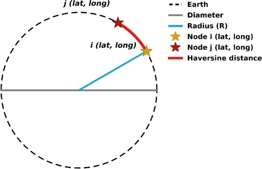
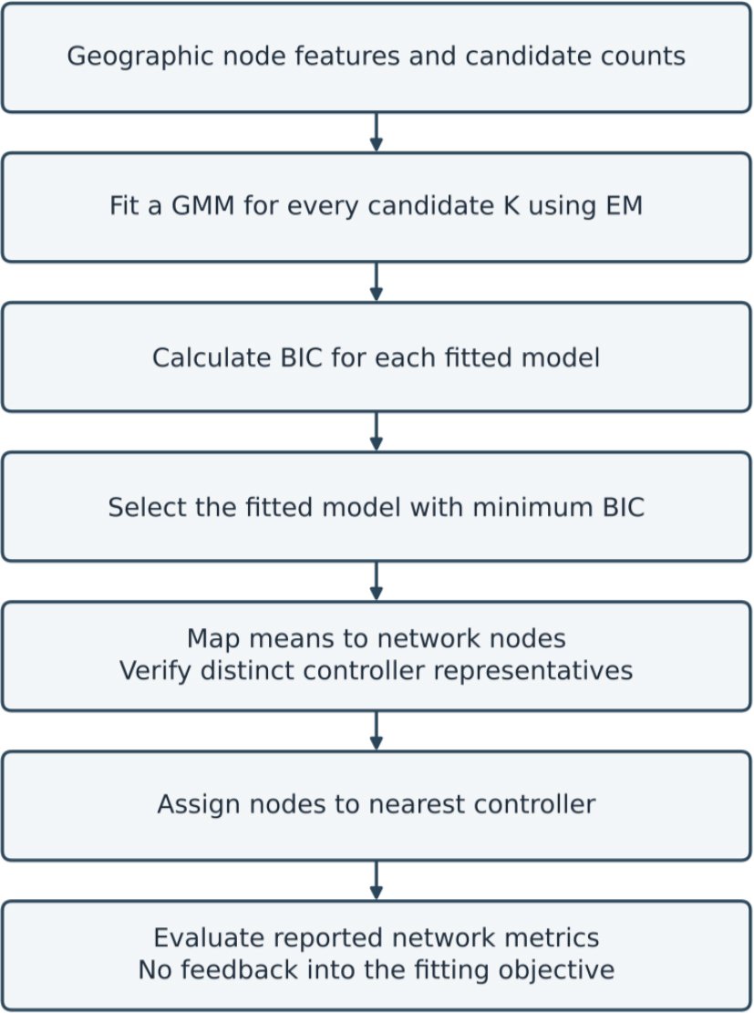
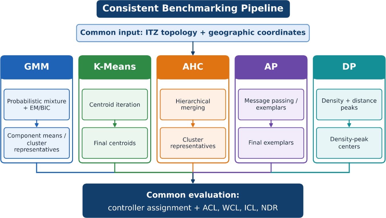
Model fitting and network evaluation are separate steps. EM fits one mixture per candidate K, BIC selects among them, and the selected means are mapped to the network nodes that host controllers. ACL, WCL, ICL and the emulation metrics are computed afterwards and play no part in the fit. Figs. (1–3) show the distance computation and the workflow.
Fig. (1). Haversine geometry used to compute geographic distance between SD-WAN nodes.
Fig. (2). Model fitting precedes BIC selection; network metrics are evaluated after placement.
Fig. (3). Common implementation and benchmarking pipeline for GMM and the four clustering baselines.
3.1. Data Preparation and Haversine Distancing
TATA, BICS and BESTEL were taken from the Internet Topology Zoo [40]. Nodes without coordinates and invalid edges were removed. Pairwise geographic separation was computed with the Haversine formula, Eq. (1) and Fig. (1) [41], which works on the sphere and so avoids the error of a planar distance over continental spans.
Dᵢⱼ = 2R arcsin √[sin²(Δφᵢⱼ/2) + cos φᵢ cos φⱼ sin²(Δλᵢⱼ/2)] (1)
Eq. (1) yields a length in the unit of R, not a delay in μs. Tables 3–5 keep the microsecond values of the original record, but that record does not name the timing instrument, the path aggregation or the distance-to-delay conversion behind these placement-stage values. They are treated as reported latency summaries, not verified WAN propagation measurements. The emulator RTTs in Table 7 are a separate reported outcome.
In Eq. (1), D_ij is the great-circle distance between nodes i and j, R the Earth radius, φ latitude and λ longitude, with Δφ_ij and Δλ_ij the differences between the two nodes. The clustering and assignment stages take these distances as their spatial basis.
3.2. GMM Mechanism
In a GMM, an unsupervised probabilistic model, each Gaussian component is a candidate controller domain. K-Means gives every observation one hard centroid and implicitly spherical clusters; a GMM estimates μₖ, Σₖ and πₖ per component, so domains may be anisotropic and may overlap. This suits SD-WAN sites that are unevenly spread or lack sharp geographic boundaries. The mixture density is Eq. (2).
p(x) = Σₖ₌₁ᴷ πₖ N(x | μₖ, Σₖ) (2)
In (2), πₖ is the mixing coefficient of component k and μₖ, Σₖ its mean and covariance, with πₖ ≥ 0 and Σₖ πₖ = 1. EM (Section 3.3) estimates the parameters, BIC (Eq. (3)) scores each candidate K, and the lowest-BIC model is kept.
BIC(K) = −2ℓ(θ̂K; X) + pK ln N (3)
For fixed K, the fitted criterion is ℓ(θ; X) = Σᵢ log[Σₖ πₖ N(xᵢ | μₖ, Σₖ)], subject to πₖ ≥ 0, Σₖ πₖ = 1 and positive-definite covariance matrices. EM seeks a local solution for θ = {πₖ, μₖ, Σₖ}. BIC(K) = −2ℓ(θ̂K; X) + pK log N then selects K̂ = arg minK∈𝒦 BIC(K), where 𝒦 is the candidate set. For unrestricted full covariance in d dimensions, pK = (K − 1) + Kd + Kd(d + 1)/2. With d = 2, pK = 6K − 1. This parameter count is conditional on full covariance; the actual covariance setting and candidate range must be recovered from the implementation. BIC balances density fit and statistical model complexity. Its penalty is not an operating-cost model and does not jointly minimise latency, imbalance or deployment cost.
3.3. Expectation-Maximization (EM)
Component membership is latent, so the parameters are estimated with EM. From initial μₖ, Σₖ and πₖ, EM alternates an E-step and an M-step until the log-likelihood gain drops below a tolerance or an iteration cap is reached.
Expectation: each node xn receives a responsibility for every component, computed from the current values of:
- Mean (μk): mean location of the component’s nodes.
- Covariance (Σk): spread and orientation of the nodes about μk.
- Mixing coefficient (πk): fraction of the network assigned to the component.
The responsibility γ(znk) of component k for node xn is given by Eq. (4):
γᵢₖ = πₖ N(xᵢ | μₖ, Σₖ) / [Σⱼ₌₁ᴷ πⱼ N(xᵢ | μⱼ, Σⱼ)] (4)
N(·) is the Gaussian density, and γ is the posterior probability that x_n belongs to component k under the current estimates.
Maximization: After assigning probabilities in the E-step, we update the clusters’ parameters to better fit the data:
- New mean (μ_k^new): Calculated as the weighted average of all nodes, where the weights are the probabilities from the E-step.
- New covariance (Σ_k^new): Updated to reflect how spread out the nodes are around the new mean.
- New mixing coefficient (π_k^new): adjusted to reflect the proportion of all data points that are likely to be in cluster k.
The formulas (Eq. 5-7) for these updates are:
(5)
(6)
(7)
Nₖ = Σᵢ γᵢₖ is the effective size of component k. EM does not decrease the likelihood between iterations but can stop at a local maximum or a degenerate covariance, which is why reproducible implementations add covariance regularisation and several initialisations. Restart count, tolerance and regularisation value are absent from the retained record and are not asserted here. Fig. (2) and Algorithm 1 state the intended procedure, which the manuscript alone does not allow to be fully reconstructed.
A fitted mean is generally not a node. Each mean is moved to the geographically nearest topology node, and each node is then assigned to the nearest selected controller, so the final domains need not match the posterior-membership domains. Two means can also map to one node.
| Algorithm 1. Statistical fitting and static controller placement |
Input: coordinates X; topology nodes V; candidate set 𝒦; EM settings. Output: selected mixture; controller nodes C; hard assignment of V to C. Procedure 1. for K ∈ 𝒦 do: θ_K ← EM(X, K) 2. BIC(K) ← Eq. (3) at θ_K // same features and covariance type for every K 3. K̂ ← arg min_K BIC(K); M ← {μ_1, …, μ_K̂} of θ_K̂ 4. C ← {arg min_{v ∈ V} D(v, μ_k) : μ_k ∈ M} // D from Eq. (1) 5. if |C| < K̂ or some c ∈ C is not deployable: apply a collision rule and report it // rule absent from the original record 6. for v ∈ V do: a(v) ← arg min_{c ∈ C} D(v, c) 7. evaluate ACL, WCL, ICL and emulation metrics on (C, a); θ_K̂ is not re-selected from them |
3.4. Clustering Metrics
ACL, WCL, ICL and NDR describe different aspects of a configuration and are not combined into an optimisation objective. Eq. (8-11) below retain the pairwise intra-domain interpretation of the original equations. In particular, intra-domain node-pair latency must not be relabelled as node-to-controller latency.
Average-case latency within domain k is the mean of the ordered node-pair delays in that domain. Let Vₖ contain nₖ nodes and let δᵢⱼ denote latency, rather than Haversine distance. For nₖ ≥ 2:
ACLₖ = [1 / (nₖ(nₖ − 1))] Σᵢ∈Vₖ Σⱼ∈Vₖ,ⱼ≠ᵢ δᵢⱼ. (8)
Worst-case latency within domain k is the largest node-pair latency for nₖ ≥ 2:
WCLₖ = maxᵢ,ⱼ∈Vₖ,ᵢ≠ⱼ δᵢⱼ. (9)
For distinct selected controller nodes cₖ and cₗ, the pairwise inter-controller latency is:
ICLₖₗ = δ(cₖ, cₗ), k ≠ l. (10)
A network-level ACL requires an explicit weighting across domains, and a network-level ICL requires a specified mean, sum or maximum across controller pairs. Singleton-domain handling must also be specified. These conventions cannot be inferred from the existing table entries. For hard assignments, NDR is defined by the maximum domain size relative to the mean:
NDR = maxₖ nₖ / (N/K) = K maxₖ nₖ / N. (11)
3.5. Computational Complexity and Scalability
Let N be the number of nodes, K the number of components, d the feature dimension, I the EM iterations and S the independent initialisations. A full-covariance EM fit costs O(I(NKd² + Kd³)), including covariance factorisation, with working memory O(NK + Nd + Kd²). Selecting among 𝒦 therefore costs O(S ΣK∈𝒦 IK(NKd² + Kd³)), rather than the cost of a single fit. With d = 2 and a bounded K, each iteration is approximately linear in N. However, materialising all pairwise geographic distances costs O(N²) time and memory. Mapping representatives and assigning nodes each require O(NK) direct distance evaluations. K-Means has an approximate per-fit cost O(INKd); covariance modelling adds work, and no measured runtime advantage is claimed for GMM.
With 33–145 nodes, the tested networks do not form a scaling benchmark. Runtime, peak memory, iteration counts, model-selection cost and coordination overhead were not recorded, so the orders above are analytical bounds only. A scaling study would need a controlled sequence of N on fixed hardware, a fixed K range and restart budget, and separate timings for preprocessing, fitting, selection and assignment. On-demand distance evaluation and a narrower 𝒦 could cut the O(N²) and per-K fitting costs; neither was benchmarked.
4. COMPARATIVE ANALYSIS
GMM is compared with K-Means, AHC, AP and DP on the same three topologies and metrics, to locate where GMM gives better placement figures and where a baseline does; no single clustering model is assumed best on every objective.
4.1. Proposed Method Implementation
All five methods were implemented in Python 3, take the same geographic topology input and are scored with the same placement metrics (Section 3.4). Fig. (3) summarises the pipeline.
Inputs are shared, but recorded controller counts are not (Table 2). Tables 3–9 therefore compare complete configurations in which algorithm, K and assignment act together, and shared inputs alone do not make this a controlled algorithm comparison. Fig. (3) shows common evaluation stages, not equal controller resources.
The benchmark has three Internet Topology Zoo networks [40]: TATA with 145 nodes and 194 edges, BICS with 84 nodes and 101 edges, and BESTEL with 33 nodes and 48 edges (Table 1, Fig. 4). Three instances make this a case study. The networks are not claimed to be the largest available, a representative sample or evidence of Internet-scale behaviour, and their layouts carry no production traffic or measured control-channel delay.
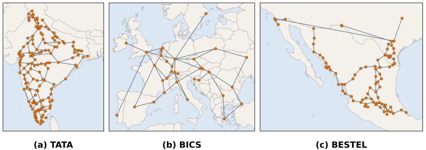
Fig. (4). Internet Topology Zoo networks used in the experiments: (a) TATA, (b) BICS, and (c) BESTEL [40].
Each topology is represented as an undirected graph G = (V, E), where V is the set of network nodes and E is the set of links. Placement metrics are computed from the controller configuration produced by each clustering method.
Table 2 gives the recorded controller count for each configuration. GMM uses BIC to select its component count. Holding K static during a run does not make comparisons across different K resource-matched. The main tables retain each method’s native count and must be read on that basis. BICS provides one existing matched-count subset: GMM, K-Means and DP each use K = 6. That subset is analysed separately in Section 5.5 and Table 10. No all-method fixed-K experiment or sensitivity sweep is available.
Tables 3–5 contain the reported placement-stage latency summaries. As explained in Section 3.4, the underlying equations describe intra-domain node-pair latency and pairwise controller latency, while their network-level aggregation is not documented. Table 3 reports GMM ACL values of 1217, 1138 and 1007 μs on TATA, BICS and BESTEL. AP is the lowest non-GMM entry in each row at 1387, 1184 and 1101 μs. These are descriptive differences between the recorded configurations, subject to the metric-provenance and controller-count limitations.
Using the lowest non-GMM ACL in each row as denominator, the GMM reductions are 12.26% on TATA, 3.89% on BICS and 8.54% on BESTEL. Table 11 identifies the comparator and controller counts for each percentage.
Table 4 shows that GMM has the lowest reported WCL on TATA (2276 μs). AP has lower WCL on BICS (2581 μs, compared with 3298 μs for GMM) and BESTEL (1814 μs, compared with 2032 μs). Relative to AP, GMM WCL is 27.78% higher on BICS and 12.02% higher on BESTEL. This counterexample prevents a claim that GMM improves every latency measure.
Table 5 reports the lowest ICL entry for GMM on each topology: 4627, 7561 and 5487 μs. Their interpretation depends on whether the network-level statistic is a sum, mean or maximum. A sum would also depend directly on the number of controller pairs. The aggregation and counts must therefore be resolved before attributing these differences solely to more favourable placement geometry.
NDR results are excluded from the performance comparison because the reported values could not be reconciled with the hard-assignment definition in (11), and the original node-to-controller assignment data were unavailable for verification. No replacement values are inferred from the aggregate summaries.
The reported latency summaries favour GMM on ACL and ICL, while AP has lower WCL on two topologies. The operational summaries are considered next.
5. RESULTS AND DISCUSSION
5.1. Simulation
The experimental record lists Mininet, Cbench and Floodlight on an Intel Core i7 host (16 GB RAM, Ubuntu 16.04 LTS, 64-bit), ten 15-second measurement cycles and a load of about 7000–68,000 host connections per switch. Not documented: the exact Cbench command and the meaning of this load parameter, link delay and bandwidth, controller versions, traffic generation, assignment logs, random seeds and baseline hyperparameters. Without execution logs, the ten cycles cannot be taken as ten independent placement replications.
5.2. Performance Metrics
Tables 6–9 hold the retained throughput (Req/s), RTT (μs), TATA utilisation and fairness summaries. The record does not say whether throughput is pooled or averaged over controllers, or how timings were collected. Utilisation and fairness follow Eqs. (12) and (13) [42]; the controller capacities and per-controller observations needed to recompute them are unavailable.
Uₖ = rₖ / qₖ, Ū(%) = (100/K) Σₖ Uₖ. (12)
J(U) = (Σₖ Uₖ)² / [K Σₖ Uₖ²], J(%) = 100 J(U). (13)
Here rₖ is the request-processing rate and qₖ is the capacity of controller k, expressed in the same units. Jain’s index is defined when at least one Uₖ is positive. Equations (12) and (13) specify the intended metrics; the retained utilisation and fairness summaries have not been independently recomputed from controller-level logs.
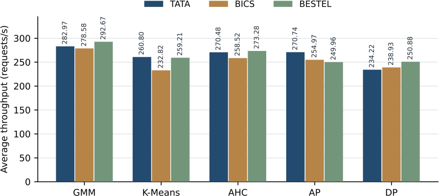
Table 6 reports throughput of 282.97, 278.58 and 292.67 Req/s for GMM on TATA, BICS and BESTEL. The strongest non-GMM comparator is AP on TATA (270.74) and AHC on BICS (258.52) and BESTEL (273.28). The corresponding increases are 4.52%, 7.76% and 7.10%, respectively. Fig. (5) presents these same reported summaries without uncertainty intervals because per-run observations are unavailable.
Fig. (5). Average throughput across the three evaluated topologies.
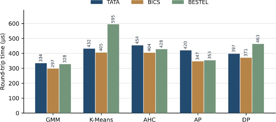
Table 7 reports GMM RTT values of 334, 297 and 328 μs on TATA, BICS and BESTEL. The next-lowest entries are DP at 397 μs on TATA and AP at 347 and 353 μs on BICS and BESTEL. The reductions are 15.87%, 14.41% and 7.08%, respectively. Fig. (6) displays the values, and Table 11 records the calculation denominators.
Fig. (6). Round-trip time across the three evaluated topologies.
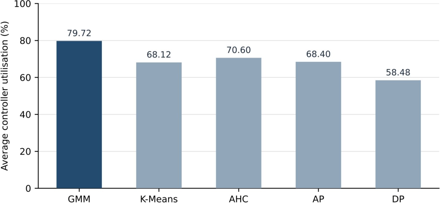
Table 8 and Fig. (7) cover TATA only. The BICS and BESTEL utilisation series were dropped: their values are identical across all five methods and could not be verified against the source data. On TATA, reported mean utilisation is 79.72% for GMM, 68.12% for K-Means, 70.60% for AHC, 68.40% for AP and 58.48% for DP. These values are descriptive, and higher utilisation is not read as an efficiency or load-balancing advantage.
Fig. (7). Reported average controller utilisation on TATA. Unverified BICS and BESTEL series are excluded.
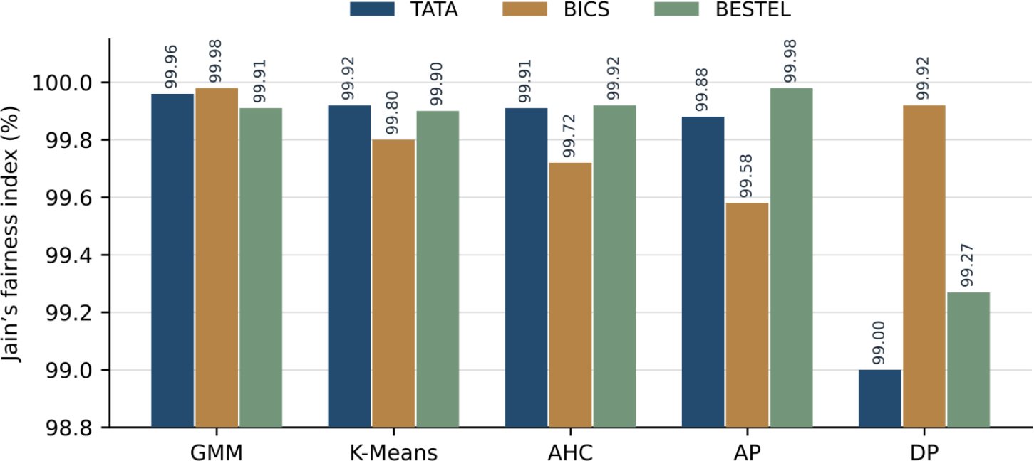
Table 9 reports Jain’s index as a percentage. GMM has the highest entry on BICS (99.98%) and TATA (99.96%). On BESTEL, AP has the highest value (99.98%), followed by AHC (99.92%), GMM (99.91%), K-Means (99.90%) and DP (99.27%). GMM exceeds the next-highest entry by only 0.06 percentage points on BICS and 0.04 percentage points on TATA, and trails AP by 0.07 percentage points on BESTEL. Such near-saturation values offer limited discrimination, and per-controller inputs are needed to validate their calculation. Fig. (8) shows the retained summaries.
Fig. (8). Jain’s fairness index across the three evaluated topologies.
Throughput and RTT favour GMM under the recorded configurations. Controller count, measurement aggregation and unrecorded settings may all contribute, so a causal effect of geographic clustering is not shown.
5.3. Statistical Interpretation
No statistical significance is claimed. Metrics from one topology share placements and measurement runs, so they are not independent replications, and maximising controller utilisation is not a universally valid ranking criterion. Sections 4 and 5 therefore report arithmetic differences only, without p-values or inferential effect sizes.
Three topology summaries and ten measurement cycles do not allow variance, confidence intervals, standardised effect sizes or corrected post-hoc tests to be reconstructed.
5.4. Limitations and Deployment Considerations
The inputs are static geographic features only, without demand, link capacity, failures or service-level requirements. Controller counts differ in most comparisons, and the K = 6 BICS subset does not replace a fixed-K sensitivity analysis. Three topologies were tested, with no measured runtime or memory scaling. Feature preprocessing, model settings, controller uniqueness, placement-latency aggregation and emulator settings cannot be reconstructed from the record. The retained summaries support a descriptive case study; statistical robustness, generalisation and deployment performance remain open.
Under changing demand, a geographically compact assignment can become unsuitable while node positions stay fixed. The procedure has no online monitoring, reassignment, controller migration or failover. An operational version would need capacity constraints, replanning triggers and limits on migration frequency, and would have to handle control-state transfer, synchronisation and transient disruption. These mechanisms and their costs lie outside the evaluated method, so the static results do not cover traffic shifts or controller failures.
5.5. Matched Controller Counts and Numerical Reconciliation
Only BICS provides a GMM comparison with identical recorded controller counts in the existing tables: GMM, K-Means and DP all use K = 6. Table 10 recalculates the differences for that subset from Tables 3–5 and 6–7. This removes the difference in controller number for these configurations, but does not establish common random seeds, equivalent tuning, verified metric aggregation or statistical robustness. There is no corresponding GMM matched-count comparator on TATA or BESTEL in Table 2.
Gain denotes 100(B − G)/B for latency and 100(G − B)/B for throughput, where B is the comparator entry and G is GMM. Positive values favour GMM. The percentages are arithmetic changes in reported summaries, not inferential effect sizes.
K G/B gives GMM and baseline controller counts. Each comparator is selected separately for its metric and topology: the lowest non-GMM latency or highest non-GMM throughput. All Table 11 comparisons have unequal K. No averaging across different physical metrics or controller budgets is performed.
CONCLUSION
GMM-based geographic clustering with BIC model selection provides an offline procedure for proposing static SD-WAN controller configurations. Across the reported TATA, BICS and BESTEL configurations, GMM has lower ACL and ICL than the evaluated alternatives, whereas AP has lower WCL on BICS and BESTEL. The reported throughput and RTT summaries also favour GMM. A BICS subset compares GMM, K-Means and DP at six controllers each, providing a limited comparison at a common controller count. These findings remain conditional on the documented measurement and configuration limitations. Inconsistent NDR results and unverified BICS/BESTEL utilisation results are excluded from the performance comparison, and no statistical or load-balancing superiority is claimed. Further evaluation should examine fixed controller budgets, verified assignments, independent repetitions and dynamic operating conditions to determine when this static planning approach offers a practical advantage.
LIST OF ABBREVIATIONS
| AP | = | Affinity Propagation |
| BIC | = | Bayesian Information Criterion |
| CPU | = | Central Processing Unit |
| DP | = | Density-Peak Clustering |
| ELA-RCP | = | Energy-Efficient and Load-Balanced Algorithm for Reliable Controller Placement |
| GMM | = | Gaussian Mixture Model |
| IoT | = | Internet of Things |
| RAM | = | Random Access Memory |
| RL-HCP | = | Reinforcement Learning-Based Heuristic Controller Placement |
| SDN | = | Software-Defined Networking |
| SD-WAN | = | Software-Defined Wide Area Network |
AUTHORS’ CONTRIBUTIONS
A.M.A. was involved in the study’s conceptualization, data collection, analysis, interpretation of findings, and preparation of the manuscript. B.O.A. contributed to data collection. Both authors reviewed the results and approved the final version of the manuscript.
ETHICAL APPROVAL AND INFORMED CONSENT
Ethical approval and informed consent were not applicable, as the study analyzed source-code data and did not involve human participants, animals, or personal data.
AVAILABILITY OF DATA AND MATERIALS
The data will be made available on reasonable request by contacting the corresponding author [A.M.A].
FUNDING
The authors received no specific funding for this study.
CONFLICT OF INTEREST
The author is a member of the Editorial Board of the Majestic Journal of Information Technology. To maintain the integrity and impartiality of the peer-review process, the author was not involved in the peer review, editorial assessment, or decision-making concerning this manuscript. The entire process was handled independently by another editor to ensure an unbiased evaluation.
ACKNOWLEDGEMENTS
The authors acknowledge the support of the Faculty of Computer Science and Information Technology (FSKTM), Universiti Putra Malaysia (UPM).
DECLARATION OF AI
ChatGPT were used solely for manuscript enhancement, including language improvement and editorial refinement. All AI-assisted modifications were carefully reviewed and verified, and full responsibility for the accuracy, originality, and integrity of the final manuscript is accepted.
REFERENCES
[1] D. Kreutz, F. M. V. Ramos, P. E. Verissimo, C. E. Rothenberg, S. Azodolmolky, S. Uhlig, “Software-defined networking: a comprehensive survey,” Proc IEEE, vol. 103, no. 1, pp. 14–76, 2015,
https://doi.org/10.1109/JPROC.2014.2371999
[2] Y. Zhang, L. Cui, W. Wang, Y. Zhang, “A survey on software defined networking with multiple controllers,” J Netw Comput Appl, vol. 103, pp. 101–18, 2018,
https://doi.org/10.1016/j.jnca.2017.11.015
[3] J. Zhao, Z. Hu, B. Xiong, M. Zheng, “Performance modelling and optimization of controller cluster deployments in software-defined WAN,” in 2019 IEEE 21st Int Conf High Perform Comput Commun, IEEE 17th Int Conf Smart City, IEEE 5th Int Conf Data Sci Syst (HPCC/SmartCity/DSS), pp. 106-113, 2019,
https://doi.org/10.1109/HPCC/SmartCity/DSS.2019.00030
[4] R. Chai, X. Yang, C. Du, Q. Chen, “Network cost optimization-based capacitated controller deployment for SDN,” Comput Netw, vol. 197, Art. no. 108326, 2021,
https://doi.org/10.1016/j.comnet.2021.108326
[5] J. Zhao, Z. Hu, B. Xiong, L. Yang, K. Li, “Modeling and optimization of packet forwarding performance in software-defined WAN,” Future Gener Comput Syst, vol. 106, pp. 412–25, 2020,
https://doi.org/10.1016/j.future.2019.12.010
[6] P. Xiao, Z. Li, S. Guo, H. Qi, W. Qu, H. Yu, “A K self-adaptive SDN controller placement for wide area networks,” Front Inf Technol Electron Eng, vol. 17, no. 7, pp. 620–33, 2016,
https://doi.org/10.1631/FITEE.1500350
[7] Z. Zhao, B. Wu, “Scalable SDN architecture with distributed placement of controllers for WAN,” Concurr Comput Pract Exp, vol. 29, no. 16, 2017,
https://doi.org/10.1002/cpe.4030
[8] E. H. Bouzidi, A. Outtagarts, R. Langar, R. Boutaba, “Dynamic clustering of software defined network switches and controller placement using deep reinforcement learning,” Comput Netw, vol. 207, Art. no. 108852, 2022,
https://doi.org/10.1016/j.comnet.2022.108852
[9] O. Adekoya, A. Aneiba, “An adapted nondominated sorting genetic algorithm III (NSGA-III) with repair-based operator for solving controller placement problem in software-defined wide area networks,” IEEE Open J Commun Soc, vol. 3, pp. 888–901, 2022,
https://doi.org/10.1109/OJCOMS.2022.3172551
[10] Y. Jimenez, C. Cervello-Pastor, A. J. Garcia, “On the controller placement for designing a distributed SDN control layer,” in 2014 IFIP Netw Conf, pp. 106-113, 2014,
https://doi.org/10.1109/IFIPNetworking.2014.6857117
[11] Z. Guo, C. Li, Y. Li, S. Dou, B. Zhang, W. Wu, “Maintaining the network performance of software-defined WANs with efficient critical routing,” IEEE Trans Netw Serv Manag, vol. 21, no. 2, pp. 2240-2252, 2023,
https://doi.org/10.1109/TNSM.2023.3335404
[12] K. Nguyen, S. Yamada, “An experimental feasibility study on applying SDN technology to disaster-resilient wide area networks,” Ann Telecommun, vol. 71, pp. 639–47, 2016,
https://doi.org/10.1007/s12243-016-0502-2
[13] V. Tyagi, S. Singh, “GM-WOA: A hybrid energy efficient cluster routing technique for SDN-enabled WSNs,” J Supercomput, vol. 79, no. 13, pp. 14894–922, 2023,
https://doi.org/10.1007/s11227-023-05263-7
[14] G. Ramya, R. Manoharan, “Traffic-aware dynamic controller placement in SDN using NFV,” J Supercomput, vol. 79, no. 2, pp. 2082–107, 2022,
https://doi.org/10.1007/s11227-022-04717-8
[15] N. Sanoussi, K. Chetioui, G. Orhanou, S. El Hajji, “ITC: Intrusion tolerant controller for multicontroller SDN architecture,” Comput Secur, vol. 132, Art. no. 103351, 2023,
https://doi.org/10.1016/j.cose.2023.103351
[16] J. Ordonez-Lucena, P. Ameigeiras, D. Lopez, J. J. Ramos-Munoz, J. Lorca, J. Folgueira, “Network slicing for 5G with SDN/NFV: concepts, architectures, and challenges,” IEEE Commun Mag, vol. 55, no. 5, pp. 80–87, 2017,
https://doi.org/10.1109/MCOM.2017.1600935
[17] S. Bera, S. Misra, A. V. Vasilakos, “Software-defined networking for Internet of Things: a survey,” IEEE Internet Things J, vol. 4, no. 6, pp. 1994–2008, 2017,
https://doi.org/10.1109/JIOT.2017.2746186
[18] S. Jain, A. Kumar, S. Mandal, J. Ong, L. Poutievski, A. Singh, a. l. et, “B4: experience with a globally-deployed software defined WAN,” in Proc ACM SIGCOMM 2013 Conf, pp. 3–14, 2013,
https://doi.org/10.1145/2486001.2486019
[19] C. Scarpitta, G. Sidoretti, A. Mayer, S. Salsano, A. Abdelsalam, C. Filsfils, “High performance delay monitoring for SRV6 based SD-WANs,” IEEE Trans Netw Serv Manag, vol. 21, no. 1, pp. 1067-1081, 2024,
https://doi.org/10.1109/TNSM.2023.3300151
[20] T. Shozi, S. Dlamini, P. Mudali, H. Kobo, “SDN-enabled switch placement in multi-domain hybrid SD-WAN,” in 2019 IEEE AFRICON, pp. 1-7, 2019,
https://doi.org/10.1109/AFRICON46755.2019.9133813
[21] C. N. Sminesh, E. G. Kanaga, A. Roy, “Optimal multi-controller placement strategy in SD-WAN using modified density peak clustering,” IET Commun, vol. 13, no. 20, pp. 3509–3518, 2019,
https://doi.org/10.1049/iet-com.2019.0124
[22] H. Kuang, Y. Qiu, R. Li, X. Liu, “A hierarchical K-means algorithm for controller placement in SDN-based WAN architecture,” in 2018 10th Int Conf Meas Technol Mechatronics Autom (ICMTMA), pp. 263-267, 2018,
https://doi.org/10.1109/ICMTMA.2018.00070
[23] N. Cai, Y. Han, Y. Ben, W. An, Z. Xu, “An effective load balanced controller placement approach in software-defined WANs,” in MILCOM 2019 – 2019 IEEE Military Commun Conf (MILCOM), pp. 263-267, 2019,
https://doi.org/10.1109/milcom47813.2019.9020804
[24] K. Yang, D. Guo, B. Zhang, B. Zhao, “Multi-controller placement for load balancing in SDWAN,” IEEE Access, vol. 7, pp. 167278–89, 2019,
https://doi.org/10.1109/ACCESS.2019.2953723
[25] C. Xiao, J. Chen, X. Qiu, D. He, H. Yin, “Goka: A network partition and cluster fusion algorithm for controller placement problem in SDN,” J Circuits Syst Comput, vol. 32, no. 9, Art. no. 2350144, 2022,
https://doi.org/10.1142/S021812662350144X
[26] M. Hassan, M. A. Gregory, S. Li, “Multi-domain federation utilizing software defined networking—A review,” IEEE Access, vol. 11, pp. 19202–19227, 2023,
https://doi.org/10.1109/ACCESS.2023.3242687
[27] C. Xu, C. Xu, B. Li, S. Li, T. Li, “Load-aware dynamic controller placement based on deep reinforcement learning in SDN-enabled mobile cloud-edge computing networks,” Comput Netw, vol. 234, Art. no. 109900, 2023,
https://doi.org/10.1016/j.comnet.2023.109900
[28] J. Ali, M. J. F. Alenazi, “Effective controller placement in software-defined Internet-of-Things leveraging Deep Q-Learning (DQL),” Comput Mater Contin, vol. 81, no. 3, pp. 4015–4032, 2024,
https://doi.org/10.32604/cmc.2024.058480
[29] M. A. Bagha, K. Majidzadeh, M. Masdari, Y. Farhang, “ELA-RCP: An energy-efficient and load balanced algorithm for reliable controller placement in software-defined networks,” J Netw Comput Appl, vol. 225, Art. no. 103855, 2024,
https://doi.org/10.1016/j.jnca.2024.103855
[30] A. Ram, S. K. Chakraborty, U. Chatterjee, “RL-HCP: A reinforcement learning-based heuristic controller placement algorithm for dynamic SDN environments,” Appl Soft Comput, vol. 186, no. Pt A, Art. no. 113997, 2026,
https://doi.org/10.1016/j.asoc.2025.113997
[31] R. Farahi, A. Ghaffari, N. Derakhshanfard, S. Taghipoureivazi, “DeepWK-MSTC: a novel approach for adaptive controller placement in software-defined networks via deep learning,” J Supercomput, vol. 82, Art. no. 174, 2026,
https://doi.org/10.1007/s11227-026-08313-y
[32] A. Chentouf, Z. Chiba, M. Miyara, “Embedding-based K-Means for multi-controller placement in software-defined networks: a cross-scale empirical study on Internet Topology Zoo,” Network, vol. 6, no. 3, Art. no. 63, 2026,
https://doi.org/10.3390/network6030063
[33] A. M. Abdulghani, A. Abdullah, A. R. Rahiman, N. A. W. Abdul Hamid, B. O. Akram, “Network-aware Gaussian mixture models for multi-objective SD-WAN controller placement,” Electronics, vol. 14, no. 15, Art. no. 3044, 2025,
https://doi.org/10.3390/electronics14153044
[34] A. M. Abdulghani, A. Abdullah, A. R. Rahiman, N. A. W. Abdul Hamid, B. O. Akram, “Dynamic multi-objective controller placement in SD-WAN: a GMM-MARL hybrid framework,” Network, vol. 5, no. 4, Art. no. 52, 2025,
https://doi.org/10.3390/network5040052
[35] B. Zhao, Y. Zhong, A. Ma, L. Zhang, “A spatial Gaussian mixture model for optical remote sensing image clustering,” IEEE J Sel Top Appl Earth Obs Remote Sens, vol. 9, no. 12, pp. 5748–59, 2016,
https://doi.org/10.1109/JSTARS.2016.2546918
[36] C. M. Weber, D. Ray, A. A. Valverde, J. A. Clark, K. S. Sharma, “Gaussian mixture model clustering algorithms for the analysis of high-precision mass measurements,” Nucl Instrum Methods Phys Res A, vol. 1027, Art. no. 166299, 2022,
https://doi.org/10.1016/j.nima.2021.166299
[37] Y. Li, J. Zhang, Z. Ma, Y. Zhang, “Clustering analysis in the wireless propagation channel with a variational Gaussian mixture model,” IEEE Trans Big Data, vol. 6, no. 2, pp. 223–32, 2020,
https://doi.org/10.1109/TBDATA.2018.2840696
[38] F. Louzada, D. C. Nascimento, O. A. Egbon, “Spatial statistical models: An overview under the Bayesian approach,” Axioms, vol. 10, no. 4, Art. no. 307, 2021,
https://doi.org/10.3390/axioms10040307
[39] M. Zhang, A. Parnell, “Review of clustering methods for functional data,” ACM Trans Knowl Discov Data, vol. 17, no. 7, Art. no. 91, pp. 1–34, 2023,
https://doi.org/10.1145/3581789
[40] Knight S, Nguyen HX, Falkner N, Bowden R, Roughan M. “The Internet Topology Zoo.” IEEE Journal on Selected Areas in Communications. vol. 29, no. 9, pp. 1765–1775, 2011,
https://doi.org/10.1109/JSAC.2011.111002
[41] Kettle S. Distance on a sphere: The haversine formula [Internet]. Esri Community; 2021 Dec 12 [cited 2023 Dec 15]. Available from: https://community.esri.com/t5/coordinate-reference-systems-blog/distance-on-a-sphere-the-haversine-formula/ba-p/902128
[42] H. S. Bin-Obaid, T. B. Trafalis, “Fairness in resource allocation: foundation and applications,” in Springer Proc Math Stat, 2020., pp. 3–18. 2020,
https://doi.org/10.1007/978-3-030-37157-9_1
Licensed
© 2026 Copyright by the Authors.
Licensed as an open access article using a CC BY 4.0 license.
Article Contents Author Abdulrahman Mawlood Abdulghani1, * , Bilal Omar Akram1 1Department of Communication Technology and Network, Faculty of Computer
Article Contents Author Ananya Mishra1, * 1GIFT Engineering and Management College, GIFT Autonomous, Bhubaneswar, India Article History: Received: 13 June,
Article Contents Author Snehal Bansod1, * 1Department of Oral and Maxillofacial Surgery, Maitri Educational Society, Chhattisgarh, India Article History: Received:
Article Contents Author Shallu Kadiyan1, Anupreet Kaur Sobti1 , Ritu Pradhan1 , Vasudha Bansal1, * 1Department of Foods and Nutrition,
Article Contents Author Hafsah Khan1, * , Ayesha Farooq1 , Muhammad Sohail1 , Palwasha Abrar Hussain1 ,
Article Contents Author Ajay Mahesh Gaur1, * 1University of Colorado Denver, Denver, USA Article History: Received: 30 July, 2026 Revised:


PDF