

















CM Publisher

Majestic American Journal of Mathematics and Physics

Article Contents

Article ID: CM2601109004

Views: 79
Volume 1 (2026)
Published 07 Nov 2026

Constrained Deep Operator Networks with a Fully Discrete Error Bound for a Material-Coordinate Fractional-Diffusion Benchmark

📚 Cited by: 0

⬇ Downloads: 1


Author

1Department of Mathematics, University of Central Punjab, Lahore, Pakistan

Article History:

Received: 25 September, 2026

Revised: 09 October, 2026

Accepted: 14 October, 2026

Published: 07 November, 2026

ABSTRACT:

Introduction: Variable-order fractional diffusion can model heterogeneous memory but remains costly in many-query studies. This work treats a prescribed moving-interval benchmark formulated in a fixed material coordinate, not a general Eulerian moving-boundary fractional PDE. All claims are restricted to this linear, one-dimensional, fully discrete benchmark.

Methodology: A constrained physics-informed Deep Operator Network (CP-DON) was developed for this material-coordinate benchmark. The architecture combines an exact trial map for the initial condition, homogeneous endpoints and non-negativity with a residual regulariser evaluated using the chosen 32×20 variable-order L1 discretisation of the reference solver. Thus, the residual enforces consistency with that fully discrete benchmark rather than with the continuum fractional PDE directly. The trial map is deliberately restrictive: the prediction stays zero wherever the initial profile is zero, so the map cannot represent every admissible solution. A residual/smallest-singular-value bound provides a deterministic, case-specific error bound relative to the assembled discrete system; it is not a continuum-error certificate. Discretisation convergence was examined by nested grid refinement, and training was repeated with five additional random seeds.

Results: CP-DON achieved mean relative L2 errors of 0.0071, 0.0100 and 0.0192 under interpolation, fractional-order shift and geometry-shift tests, reducing unconstrained DeepONet error by 58.4%, 57.9% and 41.7% in the reported single-seed run (61.2 ± 4.3%, 56.3 ± 3.6% and 41.5 ± 4.0% over five additional seeds). The audited bound was satisfied in all 60 audited cases, with mean efficiency indices from 8.73 to 16.06 (case-wise medians 8.86–15.70). The reported 61.7-fold acceleration is an inference-only benchmark under the specified CPU setting (batched neural evaluation against a per-case solver loop) and excludes certificate/SVD, training and data-generation costs; the explicit SVD certificate was about 50 times more expensive than a solve in a re-measurement. The 32×20 benchmark itself differs from a 992×608 reference by 1.7–2.0% (relative L2).

Conclusion: In the single-seed ablation, exact structural encoding explained about 87% of the in-distribution absolute improvement over DON; residual regularisation contributed about 13%. Over five further seeds the structural share was 82 ± 9%, and under an equal 140-epoch cap CP-DON improved on C-DON in only 2 of 5 seeds, so the residual benefit is not established independently of the longer training. Geometry-shift final-time error remained above 5%, so the method is a controlled parameter-range surrogate with a conservative warning signal, not a general moving-boundary solver. The framework integrates admissibility constraints, discrete residual training and a fully discrete error bound for repeated solves within a known benchmark family; the bound controls error only relative to the fully discrete 32×20 system, not the continuum solution. Its practical role is an accept-or-solve workflow in which large certificates trigger a numerical solve or training-set expansion.

Keywords: Variable-order fractional diffusion, DeepONet, neural operator, material coordinate, moving-interval benchmark, posteriori error bound, structure-preserving learning, scientific machine learning, numerical analysis.

1. INTRODUCTION

Fractional differential equations are more and more employed when the transport, relaxation or diffusion depends not merely on the current state, but also on the non-local past. A complementary computational approach is provided by scientific machine learning, which uses a learned map to replace repeated high fidelity solves, but retains selected physical and/or mathematical information [1, 2]. This opportunity is attractive for parameter studies, inverse problems, uncertainty analysis, and design loops, but sets up a second requirement on top of the predictive accuracy of the surrogate: it must be admissible and the error must be assessable for each query.

One particular challenge is the variable order time-fractional diffusion. The order may be a memory law which varies with time, location, or state of materials, so that the history kernel varies during the simulation. Recent analysis has established maximum principles and regularity properties for variable-order models [3], while finite-element studies have provided optimal-order estimates without imposing unrealistic smoothness on the exact solution [4]. Fast finite-element and robust time-stepping methods have subsequently reduced the cost of multidimensional and low-regularity problems [5, 6]. Multi-term formulations [7], variable-order advection–reaction–subdiffusion models [8], and high-order variable-exponent diffusion-wave schemes [9] further demonstrate that the numerical-analysis literature is moving toward increasingly heterogeneous memory laws. Nevertheless, a new linear system or history update is still required for every parameter instance.

Neural approaches to fractional dynamics have advanced rapidly during 2024–2025. Neural variable-order differential-equation networks learn changing memory orders directly from data [10, 11]. The physics-informed formulations for fractional differential equations have also been created, such as optimisation-based methods [12] and spectrally adapted networks [13]. These studies show that this is possible, but the majority of them consider a single solution in a specific family of solutions and neglect the moving geometry while also not providing an independently computable error certificate.

Neural operators focus more directly on the many-query problem by learning a mapping between function spaces. The Fourier Neural Operator (FNO) has demonstrated the ability of spectral parameterisation to learn families of parametric partial differential equations [14] while DeepONet has been able to learn nonlinear operators as a separable representation through branch and trunk networks [15]. Kovachki et al. [16] merged a general neural-operator framework with approximation theory. Comparative evidence shows that the architecture choice, geometry, noise, and data representation have a significant impact on accuracy, and that the behavior of DeepONet and FNO can vary outside simple benchmark settings [17]. The key observations lead to a model with an inductive bias that is more appropriate to the class of admissible solutions than just relying on unconstrained regression.

Geometry generalisation is a well-established challenge for neural operators. Geo-FNO maps irregular physical domain onto a latent regular grid [18]. Diffeomorphism Neural Operators also map a variable domain problem to a reference domain [19]. There are several variants of the physics-informed geometry-aware neural operators that integrate geometry encoders into the physics-informed training [20], and point-cloud operators that extend this framework to unstructured and topologically varying discretisations [21]. These techniques give strong evidence that geometry generalisation is possible, but it is more challenging than interpolation over familiar domains and the methods for measuring uncertainty reported so far are mostly empirical and not rigorous.

A second line of work uses governing equations during operator training. Physics-Informed Neural Operators combine data at one resolution with equation constraints at another [22]. A variational Physics-Informed Neural Operator reduces the dependence upon labelled data by leveraging energy forms [23]. Multiwavelet operators feature the implementation of bases over multiple scales [24] and message-passing neural PDE solvers have been developed using local graph interactions for temporal systems [25]. This work likewise reinforces operator learning with a residual based on a discrete physics model, but computes the residual using the variable-order L1 history operator employed by the reference discretisation.

Structural restrictions are also crucial. Unlike soft penalties, exact constructions based on distance functions or trial functions can remove incompatible functions from the hypothesis space more effectively [26]. This is important as physics-informed optimisation has been shown to have gradient imbalance issues [27] and identifiable failure modes when the residual is not well-scaled or when frequencies in the target are problematic [28]. Here the initial value, homogeneous endpoints and non-negativity are enforced by construction. The approach thus avoids selecting three penalty weights and yields non-negative concentrations without post-processing.

Moreover, reliable deployment needs more than a typical test error. Berrone et al. [29] present a reliable and efficient a posteriori estimator for variational physics-informed neural networks (PhysicsNN) for elliptic boundary-value problems. The related works are a priori and a posteriori analysis for the Deep Ritz method [30], a neural-network recovery-type a posteriori estimator of finite-element diffusion solutions [31], multigoal-oriented dual-weighted-residual error estimation for physics-informed neural networks (PINNs) [32], and an extended Galerkin neural-network framework for variational problems with error control [33]. These are different styles of error-control constructions, not certificates to swap, but they do show an increase in interest in rigorous or computable error evaluation of scientific machine learning. Neural operator simulations can speed up simulations by orders of magnitude [34] and recent out-of-distribution studies reveal that neural operators can take a hit when parameters shift [35]. This distinction between interpolation and true generalisation is also emphasized for reduced-order and neural methods for parametric PDEs [36].

Against this background, the study asks whether a constrained operator surrogate can be paired with a directly computable, case-wise discrete error bound for a variable-order fractional-diffusion benchmark with parameter-varying interval length. The novelty is not the linear-algebra inequality in Proposition 2 itself, which is standard, but its integration into the constrained operator-learning workflow as a case-wise screening mechanism. Relative to residual-based a posteriori estimators for neural solvers [29, 32, 33], which are derived for variational (typically elliptic or goal-oriented) formulations, the present bound (i) applies to the non-symmetric, history-dependent system generated by the variable-order L1 scheme, (ii) needs only the assembled matrix and the surrogate output, with no reference solution, and (iii) can be applied to any surrogate output, here one that already satisfies the initial, boundary and sign conditions. Its limitations are equally explicit: it controls only the error with respect to the discrete system, it requires σmin(A), and it is conservative. The contributions are: (1) a methodological contribution, namely a constrained operator architecture that integrates exact initial, boundary and positivity conditions with a residual evaluated under the same chosen 32×20 variable-order L1 discretisation as the reference solver; (2) a reliability contribution, namely a directly computable case-specific upper bound for error relative to the fully discrete reference system; (3) an empirical contribution, namely a controlled ablation that separates exact constraints from residual regularisation across interpolation, fractional-order-shift and geometry-shift regimes; and (4) a scope contribution, namely an explicit distinction between interpolation, parameter-range extrapolation and the harder geometry-shift setting. The trial map is deliberately restrictive (Section 2.3): it cannot represent solutions that become non-zero where the initial profile vanishes. The scope of all claims is a one-dimensional, linear, synthetic benchmark with one discretisation, in which interpolation and parameter-range extrapolation, not distributional robustness, are tested. All outputs are supplied for reproduction.

2. MATERIALS AND METHODS

2.1. Prescribed Moving-Interval Benchmark in a Material Coordinate

Let the physical interval be x in (0,L(t)), where L(t)>0 is prescribed, and define the material (reference) coordinate y=x/L(t) in (0, 1). The benchmark is formulated directly in this material coordinate. It is therefore a fixed-domain memory-diffusion model with the time-dependent coefficient κ/L(t)², rather than a general Eulerian moving-boundary fractional diffusion equation with an additional transport term. The unknown u(y,t) is interpreted as a non-negative material concentration or temperature-like field. For final time T=1, the model is

   (1)

   (2)

The time-dependent Caputo-type order is α(t)=α₀+αa sin(πt), clipped to [0.35, 0.97], and L(t)=L₀(1+ρt). The coefficient κ is constant in time but is sampled independently for each case. The geometry enters only through the coefficient κ/L(t)² in the material-coordinate system. The expansion and contraction parameter shifts are generated within this design, which does not assert equivalence to a general Eulerian moving-boundary PDE. The first profiles were created to be

   (3)

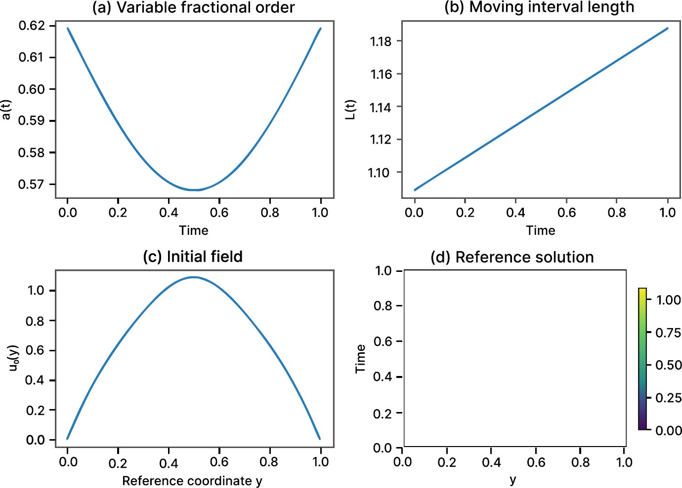
The ranges in Table 1 preserve non-negative, smooth profiles. In (3), A>0 and y(1-y)≥0; moreover, the bracketed shape factor is bounded below by 1−|c₁|−|c₂|≥0.70 for the permitted ranges, even when c₁ and c₂ are negative. Negative numerical round-off was clipped to zero in the data generator. Table 1 lists the parameter ranges, and Fig. (1) illustrates a representative fractional order, interval length, initial field and fully discrete reference trajectory.

Table 1. Dataset composition and parameter ranges for the material-coordinate benchmark.

QuantityTraining / In-DistributionFractional-Order Shift TestMoving-Geometry Shift Test
Initial amplitude A0.80–1.200.80–1.200.80–1.20
Shape coefficient c₁−0.18–0.18−0.18–0.18−0.18–0.18
Shape coefficient c₂−0.12–0.12−0.12–0.12−0.12–0.12
Base order α₀0.56–0.860.44–0.52 or 0.90–0.950.56–0.86
Order amplitude αa−0.08–0.08−0.05–0.05−0.08–0.08
Initial length L₀0.82–1.180.82–1.180.65–0.76 or 1.26–1.40
Length rate ρ−0.18–0.18−0.18–0.18−0.34–−0.24 or 0.24–0.34
Diffusivity κ0.035–0.1200.035–0.1200.035–0.120
Cases320 train + 64 validation + 80 test80 test80 test

Fig. (1). Representative benchmark case: (a) Variable fractional order, (b) Moving interval length, (c) Non-negative initial field, and (d) Fully discrete reference solution.

2.2. Variable-Order L1 Reference Discretisation

A uniform grid with Nx=32 spatial nodes and Nt=20 temporal levels was used for the main dataset. Let Δy=1/(Nx−1), Δt=T/(Nt−1), and αn=α(tn). The variable-order Caputo derivative at time tn was approximated by the L1 history sum.

   (4)

   (5)

The spatial second derivative used the centred three-point stencil. At every time level, the resulting tridiagonal system was solved by a banded direct solver. This approach is consistent with recent robust and high-order analyses of variable-order fractional equations [4, 9] and with contemporary numerical schemes for time-fractional reaction–diffusion problems [37, 38]. Negative round-off artefacts were clipped to zero only in the numerical data generator; the learned models were evaluated without output clipping.

An initial convergence audit used 12 in-distribution parameter cases. Solutions on 32×20 and 64×40 grids were interpolated against a 128×80 numerical reference. The mean relative errors were 0.0122 and 0.0044, respectively, with a mean error ratio of 2.80. This audit used non-nested grids and an interpolated numerical reference, so it supports refinement consistency only. It was therefore supplemented by a nested-grid refinement study and by a comparison with an exact solution (Section 3.6), which show first-order convergence of the scheme and a 32×20 discretisation error of 1.7–2.0% (relative L2). All surrogate errors and certificates reported below are relative to the 32×20 discrete problem, not to the unknown continuum solution, and no result should be read as a continuum-error estimate.

2.3. Operator Architecture and Exact Trial Map

Restriction of the trial map because the prediction is the product of u₀(y) and a positive exponential factor, the representation is a strong structural restriction, not a general parameterisation. Wherever u₀(y)=0 the solution remains zero for all t, so source-driven problems, sign-changing solutions, diffusion into an initially zero interior region and non-homogeneous boundaries lie outside the representable class (see also Section 4.1). The map is appropriate here only because the generated profiles are strictly positive in the interior.

The branch input concatenated the 32 sampled values of u₀, the 20 values of α(t), the 20 values of L(t), and the scalar κ, producing a 73-dimensional vector. Inputs were standardised using training-set statistics. The trunk input was the coordinate pair (y,t) at each of the 640 grid points. Both branch and trunk encoders contained four fully connected layers of width 128 and produced 72 latent coefficients. The unconstrained DeepONet output was the branch–trunk inner product plus a learned scalar bias [15].

For the constrained models, the raw operator output zθ was embedded in the trial map

   (6)

with the exponent restricted to [−8, 4] for numerical stability. In scalar form, the constrained output is ûθ(y,t)=u₀(y)exp(t zθ(y,t)), so the initial profile must already satisfy the homogeneous endpoint condition and non-negativity. The stored endpoint values were also set to zero after evaluation to suppress floating-point leakage. Accordingly, the endpoint RMSE reported below is a structural/postprocessing diagnostic of the implemented trial representation, not independent evidence from freely evaluated boundary predictions. The map is intentionally restrictive: wherever u₀(y)=0, the prediction remains zero for all t, so it cannot represent every non-negative diffusion trajectory. In this dataset the generated profiles are strictly positive in the interior and zero only at the endpoints, which makes the restriction compatible with the benchmark family.

Proposition 1 (admissibility of the trial representation). If , then the trial map in (6) satisfies  for every finite zθ.

Proof. At t = 0, the exponential factor equals one. At either endpoint, multiplication by u₀ gives zero. The exponential is strictly positive, so multiplication by a non-negative initial profile cannot produce a negative value. Fig. (2) shows where this constrained map enters the CP-DON workflow. The proposition is a representation property of the trial map, not a claim that the map spans all admissible non-negative solutions.
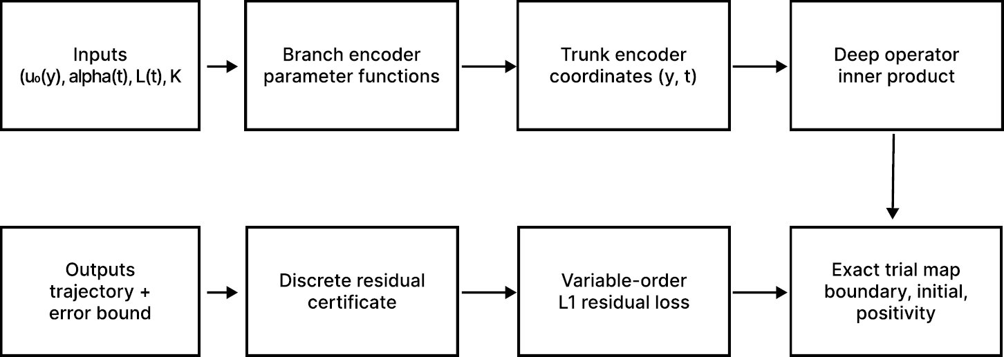
Fig. (2). End-to-end workflow of the constrained physics-informed deep operator network and the discrete residual certificate.

2.4. Training Objectives and Ablation Models

Three models were trained to isolate the contribution of each design choice. DON was the unconstrained data-only DeepONet. C-DON used the exact trial map but no equation residual. CP-DON combined the trial map with the variable-order discrete residual. All models minimised the batch mean relative trajectory error. For CP-DON, the objective was:

   (7)

   (8)

where the L1 residual is obtained by substituting the predicted trajectory into (4) and the centred spatial stencil, and u* denotes the interior reference field. The residual regulariser enforces consistency with the chosen 32×20 L1 discretisation rather than with the continuum fractional PDE directly. Accordingly, CP-DON is trained as a surrogate for the selected fully discrete benchmark map; continuum consistency or discretisation invariance is not asserted. The physics weight was selected on validation-pilot runs before final test evaluation. It was kept small so that the residual regularised, rather than dominated, supervised learning. This reduces, but does not remove, the gradient-balancing risk documented for physics-informed networks [27, 28]. Table 2 summarises the neural-operator architecture and training configuration used for the reported experiments.

Table 2. Neural-operator architecture and training configuration.

ComponentSpecification
Branch input73 standardised values
Trunk input(y,t) on 20×32 grid
Latent modes72
Branch/trunk networks4 layers; width 128
ActivationsGELU branch; tanh trunk
OptimiserAdamW; initial learning rate 2×10⁻³
Weight decay1×10⁻⁵
ScheduleCosine annealing to 2×10⁻⁵
Batch size32
Maximum epochs140 (DON, C-DON); 170 (CP-DON; residual term slowed validation convergence, so equal-compute superiority is not claimed; CP-DON was also retrained with 140 epochs, Section 3.5)
Early stoppingPatience 30 after epoch 70
Gradient clippingGlobal norm 1.0
Physics weight2×10⁻⁴ for CP-DON (validation-pilot selection; test sets not used)
Random seed2026 for the reported run (single seed); seeds 1–5 for the robustness study (Section 3.5)

Training used 320 simulations, with 64 validation cases used for model selection and early stopping. The best validation checkpoints were retained, and Fig. (3) displays the validation histories used for the reported tests. CP-DON was given a larger maximum epoch count (170 versus 140) because the residual term slowed validation convergence. The comparison with DON and C-DON is therefore not equal-budget, and the incremental effect of the residual term must be read with this in mind. CP-DON was also retrained with the same 140-epoch cap (Section 3.5). Training cost differs further: a CP-DON epoch was about six times as expensive as a C-DON epoch because the residual is evaluated sequentially over time levels. The final best validation errors were 0.0192 for DON, 0.00955 for C-DON and 0.00813 for CP-DON. The reported main run used a single seed (2026), so the bootstrap intervals over test cases do not quantify optimisation randomness; this was assessed separately with five additional training seeds (Section 3.5).
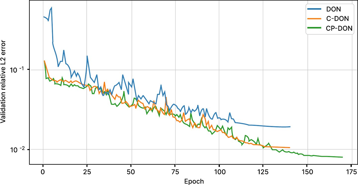
Fig. (3). Validation relative L2 error during training. Curves correspond to the best-checkpoint runs used for all reported tests.

2.5. A Posteriori Certificate for the Fully Discrete Problem

For each parameter instance μ, the interior values over all Nt−1 unknown time levels were stacked into . The variable-order L1 scheme and spatial stencil define a block lower-triangular linear system

   (9)

where z* is the fully discrete reference trajectory. Given a CP-DON prediction ẑ, the computable residual is . The smallest singular value σmin(A) is positive for the finite systems considered here because each time-step block is strictly diagonally dominant and the global matrix is nonsingular.

Proposition 2 (discrete residual certificate). The prediction error  satisfies

   (10)

Proof. Since , . By the definition of the smallest singular value, . Rearranging gives (10).

The bound is rigorous for the assembled discrete system and its mathematical validity does not require access to the reference solution. There is no circular use of the true discrete error in computing the screening quantity: the residual r=A ẑ−b is formed from the surrogate prediction and the independently assembled discrete system, while σmin(A) is determined from A. The reference trajectory z* and ||e||₂ are not components of the certificate, but are used only for purposes of the audit checking the bound satisfaction and the efficiency index. Proposition 2 is therefore not presented as a new inequality.

2.5.1. Positioning

Inequality (10) is standard. What the present workflow adds is its use as a per-query accept-or-solve test on the output of a constrained operator surrogate: a case whose bound exceeds an application tolerance is sent to the numerical solver or flagged for training-set expansion. Residual-based a posteriori estimators for variational PINNs [29] and for dual-weighted-residual and Galerkin neural frameworks [32, 33] are derived for variational problems. The bound used here instead (i) applies to the non-symmetric, history-dependent, block lower-triangular system generated by the variable-order L1 scheme, (ii) uses only the assembled matrix and the surrogate output, with no reference solution, and (iii) is model-agnostic. The price is conservatism (efficiency indices well above one), the need for σmin(A), and the restriction to the discrete problem.

2.5.2. Audit Design

The bound was evaluated on 60 cases: every fourth test case (indices 0, 4, …, 76) in each of the three test regimes, i.e., 20 per regime. The efficiency index η/||e||₂ measures sharpness: one is optimal and larger values are conservative. Because the bound is deterministic, “coverage” here only records whether the bound held for the audited case; it has no statistical (confidence-level) meaning.

2.5.3. Scope and Scalability

The bound controls the error with respect to the fully discrete system only. It is not an estimate of the continuum error, which also contains the discretisation error quantified in Section 3.6. An explicit singular value decomposition is feasible at this benchmark size (570×570) but impractical for larger systems, and its cost is excluded from the inference speed-up. A scalable version would need a cheap lower bound of σmin(A), an inf-sup estimate or a preconditioned residual majorant, as is common in residual-based a posteriori estimation [29] and neural variational error control [33].

2.6. Evaluation and Statistical Analysis

The overall result was the complete trajectory relative L2 error. Secondary outcomes included final-time relative L2 error, a relative H1 error that was discrete for the first time step, initial-condition error, endpoint root mean square error, the fraction of negative grid values, the fraction of the time steps with a mass increase greater than 10-5, normalised L1-residual RMSE, deterministic bound satisfaction and efficiency, and wall-clock inference time. Because the constrained trial map guarantees only initial data, boundary data and positivity, the mass diagnostic was treated as empirical rather than a theorem. Dispersion statistics are reported for the primary errors. Case-wise certificate efficiencies are summarised by their median, interquartile range and maximum (Table 5); per-set standard deviations of the residual and H1 error are given in the supplementary metrics file.

Mean primary errors were accompanied by 95% bootstrap confidence intervals from 2,000 resamples. The planned ablation hypothesis was directional: CP-DON was expected to lower error relative to DON and C-DON because it adds exact constraints and a residual term. Paired one-sided Wilcoxon signed-rank tests were therefore used, with zero differences discarded, the normal/asymptotic p-value approximation, no continuity correction and alternative=”less” for CP-DON minus comparator errors. Six planned pairwise tests were interpreted with Holm-Bonferroni multiplicity control. Training-seed variability was assessed by retraining all three models with five additional seeds (1–5; different initialisation and mini-batch order, identical datasets) and reporting the mean ± SD of the test-set mean errors; retraining CP-DON with the 140-epoch cap gives an equal-epoch comparison. The regimes are described as interpolation, fractional-order parameter-range extrapolation and moving-geometry parameter-range extrapolation; they are not tests of general out-of-distribution (OOD) robustness. Here “extrapolation” always means extrapolation of parameter ranges within one benchmark family; robustness to a different PDE family, initial-profile family, dimension, topology or discretisation was not tested. Runtime was averaged over 20 repeated batched neural evaluations and 20 numerical solves on the same CPU environment. The reported runtime excludes training, data generation, input standardisation overhead where outside the timed call, and certificate/SVD cost. Timing protocol: neural inference was one forward pass over the 80 in-distribution test cases (batched, PyTorch CPU, no gradient tracking), preceded by 3 warm-up passes, averaged over 20 passes and divided by 80. The numerical reference was the Python/SciPy implementation of the L1 scheme (one banded solve per time level, history sum by explicit loops, no batching across cases), timed sequentially on 20 cases. The original timings used min(8, number of cores) PyTorch threads, and their hardware identifiers were not logged. For reproducibility, timings were re-measured on an Intel Xeon (2.80 GHz, 2 vCPU) with 2 PyTorch threads, 3 warm-up passes (10 for single-case calls) and the same repetition counts (Table 6). Software versions were Python 3.13.5, NumPy 2.3.5, SciPy 1.17.0, pandas 2.2.3, PyTorch 2.10.0 (CPU) and Matplotlib 3.10.8. The experiments (additional seeds, nested-grid convergence, timing) used Python 3.13.16, NumPy 2.5.3, SciPy 1.18.1, pandas 3.0.5, PyTorch 2.14.1 (CPU execution) and Matplotlib 3.11.2; in that environment the saved checkpoints reproduced the Table 3 errors to four decimals.

3. RESULTS

3.1. Predictive Accuracy

Table 3 reports the primary errors. In distribution, CP-DON attained a mean relative L2 error of 0.0071 (95% CI 0.0064–0.0079), compared with 0.0172 for DON and 0.0084 for C-DON. The reduction relative to DON was 58.4%, and the further reduction relative to C-DON was 15.0%. The paired Wilcoxon results were W = 0, p = 3.92e−15 against DON and W = 2, p = 4.23e−15 against C-DON; these are asymptotic one-sided p-values and are interpreted under the planned Holm-Bonferroni correction across six pairwise tests. All errors in this section are relative to the 32×20 discrete reference solution; seed-to-seed variability and errors against a finer reference are given in Sections 3.5 and 3.6.

Table 3. Predictive accuracy across interpolation and extrapolation regimes.

Test RegimeModelRelative L2, Mean (95% CI)Relative H1Final-Time Relative L2
In-distributionDON0.0172 (0.0156–0.0190)0.07580.0176
In-distributionC-DON0.0084 (0.0076–0.0092)0.04080.0096
In-distributionCP-DON0.0071 (0.0064–0.0079)0.03610.0083
Fractional-order shiftDON0.0237 (0.0212–0.0262)0.08620.0251
Fractional-order shiftC-DON0.0120 (0.0107–0.0132)0.04750.0139
Fractional-order shiftCP-DON0.0100 (0.0089–0.0110)0.04130.0119
Moving-geometry shiftDON0.0329 (0.0286–0.0374)0.09820.0532
Moving-geometry shiftC-DON0.0206 (0.0176–0.0237)0.05320.0541
Moving-geometry shiftCP-DON0.0192 (0.0156–0.0232)0.04740.0514

The same ordering held under fractional-order parameter shift. CP-DON produced 0.0100 mean error, a 57.9% reduction from DON, and its relative H1 error was 0.0413 (Fig. 4). Under moving-geometry parameter shift, CP-DON remained best on the full trajectory at 0.0192, reducing DON by 41.7%. However, the final-time geometry error remained 0.0514; this was only modestly lower than DON (0.0532) and C-DON (0.0541). The boxplots in Fig. (5) therefore show both a median improvement and a wider, harder geometry-extrapolation tail.
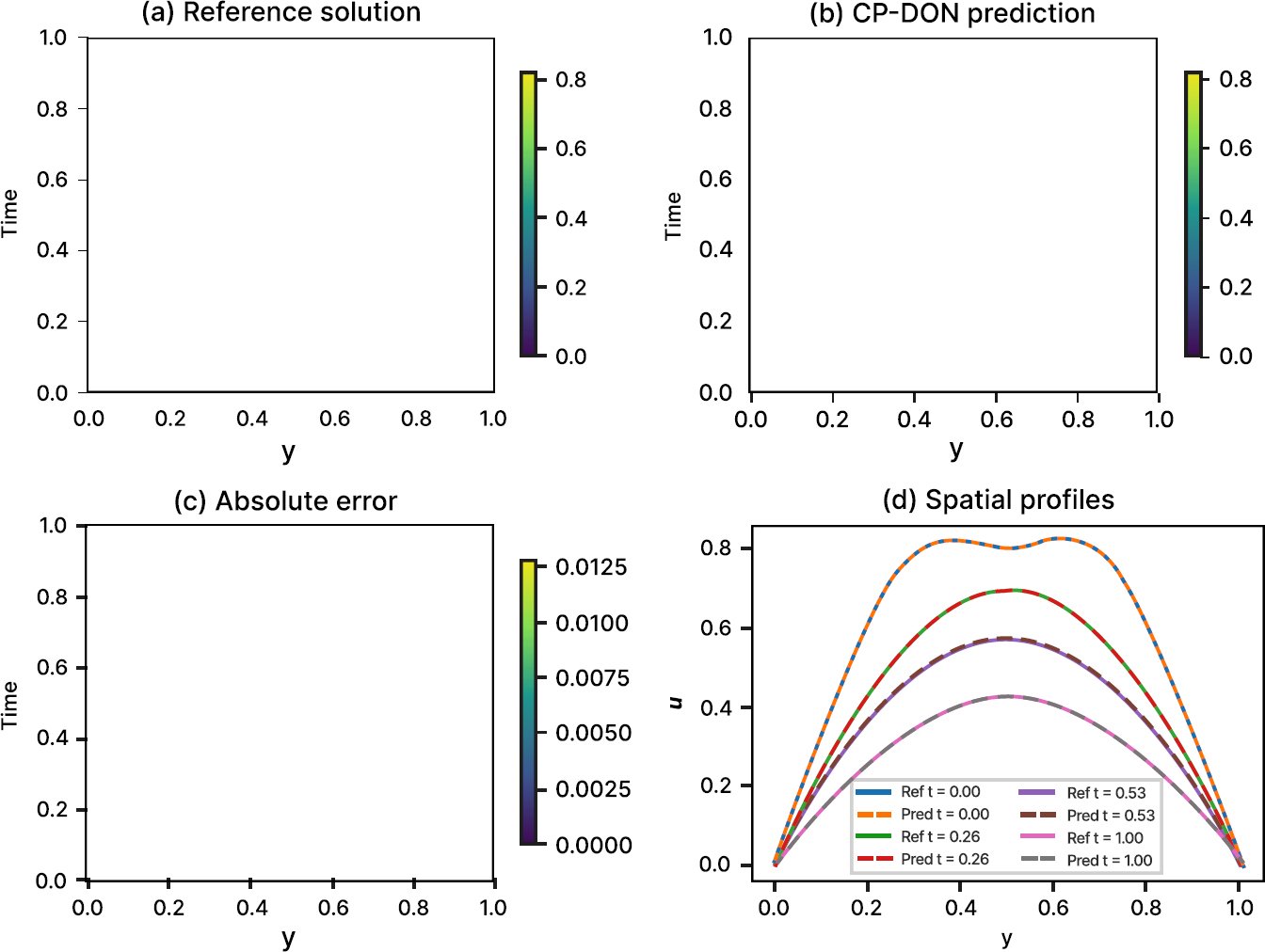
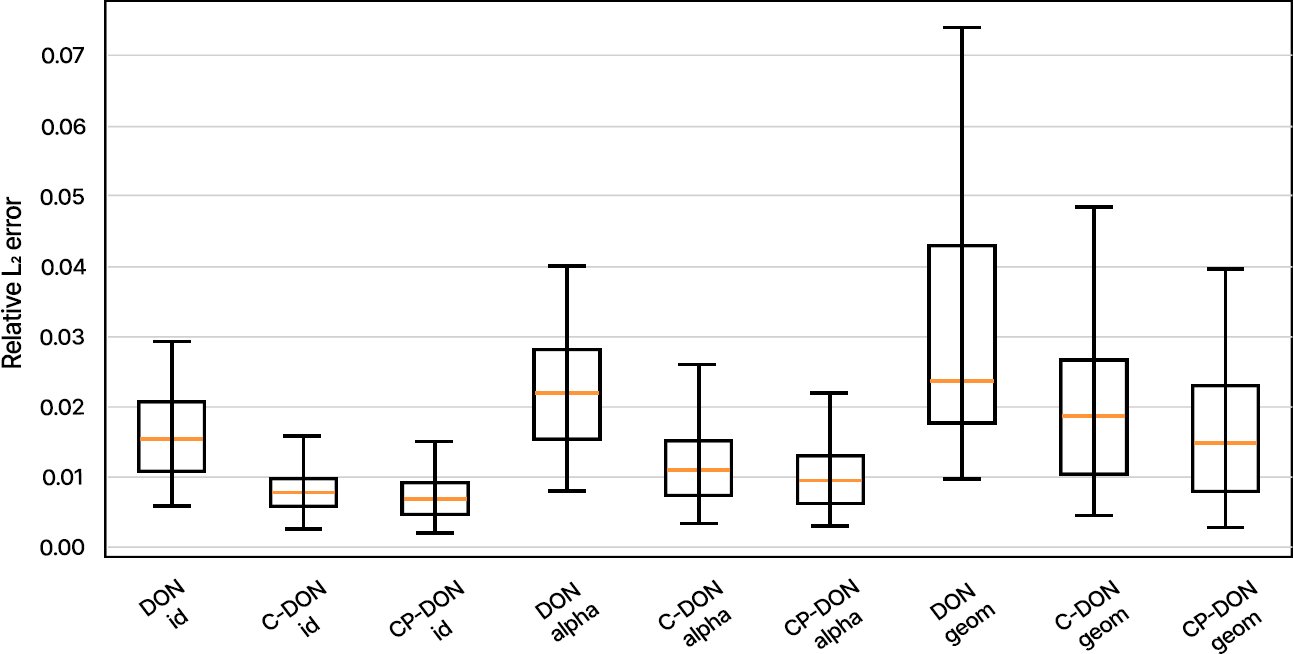
Fig. (4). Representative in-distribution CP-DON result: (a) Reference trajectory, (b) Prediction, (c) Absolute error, and (d) Selected spatial profiles.

Fig. (5). Distribution of relative L2 errors for the three models under in-distribution, fractional-order-shift, and moving-geometry-shift tests. Outliers are omitted from the boxplot display but retained in all statistics.

3.2. Exact Constraints and Discrete Residuals

The implemented trial map removed all measured violations of the three encoded structures. C-DON and CP-DON had zero initial-condition error to machine precision, zero endpoint RMSE and no negative values in every test regime. The endpoint result must be read with the implementation caveat in Section 2.3: endpoints were explicitly assigned to zero after evaluation to remove floating-point leakage. DON did not satisfy these structures: its mean initial error ranged from 0.0380 to 0.0462, endpoint RMSE from 0.0107 to 0.0141, and negative-value rate from 2.95% to 3.14% (Table 4). These failures occurred despite DON being trained directly on non-negative trajectories satisfying zero endpoints.

Table 4. Structural diagnostics and discrete physics residual.

RegimeModelInitial Rel. L2Boundary RMSENegative ValuesMass-Increase StepsNormalised Residual RMSE
In-distributionDON0.03800.01072.95%0.00%0.256
In-distributionC-DON0.00000.00000.00%0.00%0.280
In-distributionCP-DON0.00000.00000.00%0.00%0.254
Fractional-order shiftDON0.04620.01383.14%0.00%0.279
Fractional-order shiftC-DON0.00000.00000.00%0.00%0.310
Fractional-order shiftCP-DON0.00000.00000.00%0.00%0.276
Moving-geometry shiftDON0.04310.01413.05%0.53%0.438
Moving-geometry shiftC-DON0.00000.00000.00%0.00%0.408
Moving-geometry shiftCP-DON0.00000.00000.00%0.00%0.370

Residual regularisation was complementary rather than dominant. Relative to C-DON, CP-DON reduced the mean normalised residual RMSE from 0.280 to 0.254 in distribution, from 0.310 to 0.276 under fractional-order shift and from 0.408 to 0.370 under geometry shift. The decreases were around 9–11%, which is consistent with the residual term being a regulariser. Even if the admissibility of the unconstrained DON was not as good, it produced a similar residual to the one mentioned above, demonstrating that a small residual is not sufficient to satisfy initial, boundary or sign constraints.

3.3. A Posteriori Certificate

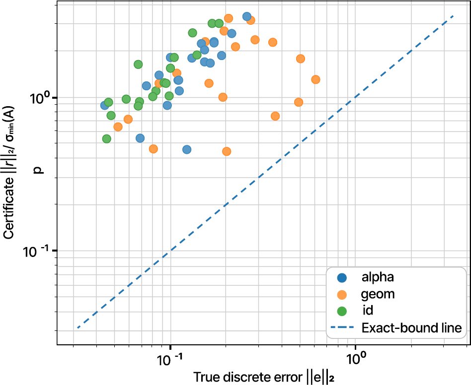
All 60 audited predictions met the deterministic bound in (10). Fig. (6) compares the certificate with the true discrete error; points above the identity line satisfy the bound. The certificate was conservative, with a mean efficiency of 16.06 in distribution, 12.66 under fractional-order shift and 8.73 under geometry shift (Table 5). The lower mean efficiency under geometry shift does not mean that these cases are easier: the true discrete error was larger, so a certificate of similar magnitude was relatively sharper. Case-wise medians were 15.70, 12.89 and 8.86, with maxima of 25.41, 19.98 and 15.63 (Table 5). Efficiency ranged from 1.87 to 25.41 across the 60 cases, so sharpness varies by an order of magnitude between cases.

Table 5. Discrete residual-certificate audit on 60 cases (deterministic bound satisfaction, not statistical coverage), with case-wise efficiency distribution.

Test RegimeAudited CasesMean True Discrete Error ||e||₂Mean Certificate ηEfficiency η/||e||₂: Mean; Median [IQR]; MaxAudited Bound Satisfied
In-distribution200.09171.462716.06; 15.70 [13.28–17.43]; 25.4120/20
Fractional-order shift200.13391.649612.66; 12.89 [9.99–15.31]; 19.9820/20
Moving-geometry shift200.23441.54408.73; 8.86 [4.79–13.11]; 15.6320/20

Note: Efficiency is defined as the certificate divided by the true discrete error ||e||₂. Case-wise values for all 60 audited cases are provided in the supplementary certificate files.

Fig. (6). Computed certificate versus true fully discrete error. The dashed identity line denotes an efficiency index of one; points above it satisfy the deterministic discrete bound for the audited case.

3.4. Geometry Extrapolation and Computational Cost

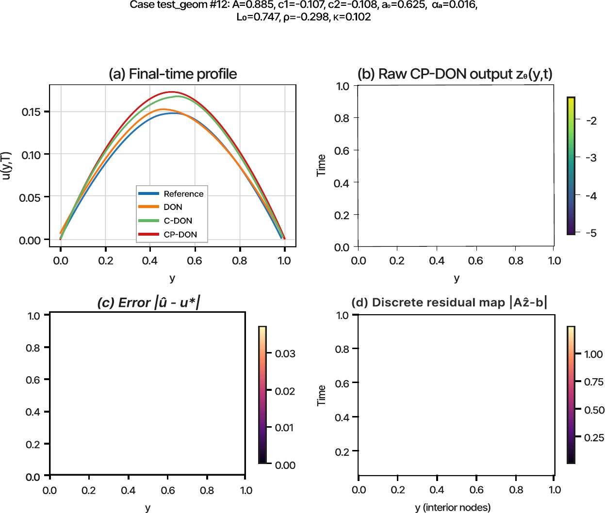
Fig. (7) gives case-level diagnostics for one unseen-geometry case (test_geom #12: L₀ = 0.747 and ρ = −0.298, so the interval contracts to L(T) = 0.524, with α₀ = 0.625 and κ = 0.102). All learned models preserved the dominant spatial mode, but the constrained models overpredicted the final-time centre amplitude (CP-DON by 16.5%; final-time relative error 0.169, against 0.055 for DON in this case). The raw output zθ (panel b) varies smoothly between −5.06 and −1.41, so the exponent clamp of [−8,4] was inactive (t·zθ ranged from −1.80 to 0). The error map (panel c) and the residual map (panel d) are largest at early times (t ≲ 0.2) and, for the residual, near the interval ends. For this case the certificate was η = 2.26 against a true discrete error of 0.357 (efficiency 6.3). One case should not be generalised, but it is consistent with Table 3: the full-trajectory error was acceptable, whereas extrapolation to different interval lengths and faster length rates remained challenging.

Fig. (7). Case-level diagnostics for a representative moving-geometry case outside the training ranges (test_geom #12; A = 0.885, c₁ = −0.107, c₂ = −0.108, α₀ = 0.625, αa = 0.016, L₀ = 0.747, ρ = −0.298, κ = 0.102): (a) Final-time profile for all models, (b) Raw CP-DON output zθ(y,t), (c) Absolute error of CP-DON, and (d) Discrete residual map |Aẑ − b| of CP-DON.

In the original timing run, batched CP-DON inference took 11.53 μs per case against 711.47 μs per 32×20 L1 solve, a ratio of 61.7. This is an inference-only benchmark under the stated CPU setting. Table 6 shows that the neural inference cost of DON and C-DON was almost the same. The comparison does not establish the speed-up of a certified CP-DON workflow, because σmin(A) computation and residual-certificate assembly were excluded. It also compares a batched forward pass over 80 cases with a sequential per-case Python solver, so the two sides do not share the same batching, threading or input-preparation assumptions. A re-measurement on documented hardware (Table 6, lower block) gave 16.7 ± 5.9 μs per case for batched CP-DON and 1270 μs per solve, a ratio of about 76. For a single-case call (batch size 1), however, the network took about 800 μs, only 1.6 times faster than the solver. Computing the certificate with an explicit SVD of the 570×570 system took about 68 ms per case, roughly 50 times the cost of a solve. On this benchmark the certified workflow is therefore slower than solving directly. The timing claim is limited to amortised, batched neural inference on the tested grid.

Table 6. Runtime and numerical-audit summary (mean per-case μs and reference-grid errors).

Method / AuditMeasured Value and Definition
DON10.95 μs per case; 80-case batched neural inference
C-DON11.60 μs per case; 80-case batched neural inference
CP-DON11.53 μs per case; 80-case batched neural inference, certificate excluded
L1 finite-difference solver711.47 μs per case; 32×20 L1 finite-difference solve
32×20 vs 128×80 reference0.0122 mean relative L2 versus a 128×80 numerical reference
64×40 vs 128×80 reference0.0044 mean relative L2 versus a 128×80 numerical reference
CP-DON + residual certificateNot timed in the original run; re-measured below
Re-measurement (Intel Xeon 2.80 GHz, 2 vCPU; 2 PyTorch threads; 3 warm-up passes; 20 repeats)Hardware and protocol for the rows below
DON, C-DON, CP-DON (batched, 80 cases)9.95 ± 2.20, 15.42 ± 2.55 and 16.68 ± 5.89 μs per case (mean ± SD over repeats)
DON, C-DON, CP-DON (single case, batch size 1)903, 963 and 801 μs per case
L1 finite-difference solver (sequential, 20 cases)1269.8 ± 23.1 μs per case
CP-DON + explicit SVD certificateAbout 68 ms per case (SVD of the 570×570 matrix about 68 ms; matrix assembly about 2 ms)

3.5. Training-Seed Robustness and Equal-Epoch Comparison

To address the single-seed limitation, all three models were retrained with five additional seeds (1–5; different initialisation and mini-batch order, identical datasets) using the settings of Table 2 (140 epochs for DON and C-DON, 170 for CP-DON). CP-DON was additionally retrained with the 140-epoch cap used for the other two models. Early stopping did not trigger in any retraining run. Table 7 reports the mean ± SD over seeds of the test-set mean relative L2 error.

Table 7. Seed-to-seed variability of the mean relative L2 error (five additional training seeds; relative to the 32×20 reference).

Test RegimeModelRelative L2,
Mean ± SD
Min–MaxReduction vs DON (%), Mean ± SDSeeds with Lower Error Than C-DON
In-distributionDON0.0181 ± 0.00150.0162–0.0203––
In-distributionC-DON0.0089 ± 0.00110.0077–0.010850.5 ± 7.5–
In-distributionCP-DON (170 epochs)0.0070 ± 0.00050.0062–0.007561.2 ± 4.35/5
In-distributionCP-DON (140 epochs)0.0095 ± 0.00210.0082–0.013347.3 ± 13.02/5
Fractional-order shiftDON0.0235 ± 0.00150.0214–0.0249––
Fractional-order shiftC-DON0.0128 ± 0.00100.0119–0.014445.4 ± 5.9–
Fractional-order shiftCP-DON (170 epochs)0.0102 ± 0.00060.0095–0.011056.3 ± 3.65/5
Fractional-order shiftCP-DON (140 epochs)0.0133 ± 0.00180.0123–0.016643.0 ± 9.42/5
Moving-geometry shiftDON0.0340 ± 0.00160.0317–0.0357––
Moving-geometry shiftC-DON0.0225 ± 0.00050.0217–0.023133.8 ± 3.6–
Moving-geometry shiftCP-DON (170 epochs)0.0199 ± 0.00090.0183–0.020541.5 ± 4.05/5
Moving-geometry shiftCP-DON (140 epochs)0.0229 ± 0.00070.0219–0.023432.7 ± 3.32/5

The ordering DON > C-DON > CP-DON (170 epochs) held in every seed and every regime. The reductions of CP-DON relative to DON (61.2 ± 4.3%, 56.3 ± 3.6% and 41.5 ± 4.0%) agree with the single-seed values of 58.4%, 57.9% and 41.7%, which lie within one standard deviation. The trial map accounted for 82 ± 9%, 80 ± 7% and 82 ± 4% of the CP-DON improvement over DON in the three regimes, consistent with the single-seed 87%.

The additional benefit of the residual term is less secure. At the 170-epoch budget CP-DON lowered the error relative to C-DON by 21.2 ± 6.0%, 19.8 ± 4.3% and 11.6 ± 2.6%. When limited to the same 140 epochs, however, CP-DON was better than C-DON in only 2 of 5 seeds in every regime (mean relative difference +5.4%, +4.0% and +1.8%, i.e., slightly worse on average). The gain attributed to the residual term therefore cannot be separated from the longer and costlier training; on the hardware a CP-DON run took about 55–70 s, against about 10 s for C-DON and 9 s for DON (seeds 3–5, uncontended). An equal-wall-clock comparison was not performed. Finally, the seed-averaged final-time geometry errors were 0.053 (DON), 0.060 (C-DON) and 0.056 (CP-DON), so the constraints did not improve the final-time error under geometry shift.

3.6. Discretisation Convergence and Continuum Context

Convergence of the L1 scheme was examined on nested grids with (Nx−1, Nt−1) = (31k, 19k) for k = 1, 2, 4, 8, 16, 32, so that every grid contains the 32×20 benchmark nodes (k = 1 reproduced the dataset solutions to within 6×10⁻⁸). For the 60 audited parameter cases the observed order, estimated at the common nodes from the differences between three successive grid levels (k, 2k, 4k), increased from 0.93 at k = 1 to 0.99 at k = 8 (case range 0.81–1.07), i.e., first-order convergence under joint refinement (Table 8). A constant-order, constant-geometry special case with initial profile sin(πy) has the exact solution u(y,t) = sin(πy)Eα(−κπ²L⁻²tα), where Eα is the Mittag-Leffler function and tα denotes t raised to the power α. For α = 0.4, 0.6, 0.8 and 0.95 the same scheme converged to it with observed orders between 0.94 and 1.08, and the relative L2 error fell from 1.4–2.7% on the 32×20 grid to 0.05–0.08% on the finest grid. The scheme therefore converges to the continuum solution at first order, but the 32×20 benchmark grid is coarse.

Table 8. Discretisation error of the 32×20 benchmark and its effect on surrogate error (992×608 reference, k = 32).

QuantityIn-DistributionFractional-Order ShiftMoving-Geometry Shift
Mean observed order p, k = 1 (60 audited cases: 20 per regime)0.920.960.90
Mean observed order p, k = 20.951.000.94
Mean observed order p, k = 40.971.010.97
Mean observed order p, k = 80.981.000.98
32×20 solution vs reference, relative L2: mean (80 test cases)0.01770.01680.0197
32×20 solution vs reference, relative L2: median [max]0.0164 [0.0338]0.0163 [0.0430]0.0134 [0.0578]
CP-DON vs 32×20 reference (Table 3)0.00710.01000.0192
CP-DON vs 992×608 reference0.02010.02220.0336
C-DON vs 992×608 reference0.02090.02320.0359
DON vs 992×608 reference0.02590.03240.0465
Mean ‖e‖₂ / η / discretisation error δ (60 audited cases)0.092 / 1.463 / 0.2060.134 / 1.650 / 0.2030.234 / 1.544 / 0.241
Audited cases with δ > ‖e‖₂20/2018/2011/20

Relative to the finer reference, the error of CP-DON is 1.8–2.8 times larger than relative to the 32×20 discrete reference (Table 8), because the training data themselves carry the discretisation error. The ranking of the three models is unchanged, so the comparative conclusions stand; what changes is the meaning of the absolute numbers. They measure how well the surrogate reproduces the 32×20 solver, not the continuum PDE. In the audited cases the discretisation error δ, measured in the same ℓ2 norm as the certificate, was 6–38% of the certificate (mean 16%) and exceeded the surrogate error in 49 of 60 cases. A combined indicator η + δ bounds the surrogate error against the finer reference by the triangle inequality, but δ is itself estimated from a finer numerical solution and is not a rigorous quantity.

4. DISCUSSION

The results support a practical but limited claim. For this material-coordinate benchmark, a constrained operator surrogate, a discrete residual loss and a residual/singular-value bound can be combined in one pipeline. The evidence is confined to the selected discrete model and parameter family, to a training procedure whose variability was quantified with only five additional seeds (Section 3.5), and to a discretisation whose own error (1.7–2.0%) exceeds the surrogate error measured against it (Section 3.6).

4.1. Exact Admissibility as an Effective Operator Bias

The main conclusion is that structural encoding was not ‘cosmetic’. C-DON lowered the in-distribution error by 51.1% relative to DON without any physics residual. In absolute terms, the trial map and the residual term contributed 0.0088 and 0.0013, respectively, about 87% and 13% of the 0.0101 DON-to-CP-DON improvement in the single-seed run. Across five further seeds the trial-map share was 82 ± 9% (80 ± 7% and 82 ± 4% under the two shifts), so the dominance of the structural component is robust, whereas the 13% residual share is uncertain (Section 4.2). The constrained models also showed no initial, boundary or sign violations in the measured data, except for the endpoint caveat in Section 2.3. The result is consistent with exact-condition approaches [26], which restrict the output class and can ease learning because the network need not approximate properties already known for the benchmark.

The result also warns against rating a scientific surrogate on trajectory error alone. The average error for DON was low, but the errors were negative at about 3% of the grid points and non-zero on the boundaries. These violations may be intolerable if u is a concentration or a probability-like value. A soft-penalty alternative would be to assign weights to initial and endpoint losses and positivity losses, and would possibly leave behind some violations. The exact map maps these properties from optimisation objectives to identities.

This restriction is fundamental, not incidental. The trial map (6) is too restrictive when the true solution changes sign, when boundaries are non-homogeneous or uncertain, when an interior zero is later filled by diffusion, or when the solution arises from a zero initial condition with a source term. The map should therefore not be applied blindly; a trial representation should instead be built to match the known admissible class.

4.2. Incremental Contribution of Physics Regularisation

The residual term added a smaller benefit once the exact constraints were imposed. In the single-seed run CP-DON lowered the error relative to C-DON by 15.0% in distribution, 16.5% under fractional-order shift and 6.7% under geometry shift, and it also lowered the normalised residual in all regimes. Over five further seeds, at the 170-epoch budget, the reductions were 21.2 ± 6.0%, 19.8 ± 4.3% and 11.6 ± 2.6%. This is not an equal-budget result: when CP-DON was limited to the 140 epochs given to C-DON, it was better than C-DON in only 2 of 5 seeds in every regime (Table 7), and a CP-DON epoch was about six times as expensive as a C-DON epoch. The residual benefit is therefore not established independently of the longer, costlier training. The trend resembles the PINO and VINO studies [22, 23], where equation information improves data efficiency or high-resolution fidelity, but the gain is modest here because the training labels are exact and λphys is small.

The ablation clarifies a point that is often confused: a physics loss and hard constraints address different problems. The trial map guarantees admissibility, whereas the residual term promotes consistency with the discrete evolution law. The normalised residual of C-DON was slightly larger than that of DON in distribution and under fractional-order shift (0.280 versus 0.256 and 0.310 versus 0.279), even though C-DON is admissible and more accurate; a small residual therefore does not imply admissibility, and admissibility does not imply a small residual. Where both are affordable, combining them is reasonable, but the present evidence supports the combination only at the cost of the longer training noted above.

The use of the discrete L1 residual also has consequences. It avoids automatic differentiation of a fractional derivative, which is costly and noisy, and it gives a training objective that matches the data generator. The regulariser is therefore a residual regulariser tied to the chosen 32×20 L1 discretisation, not to the continuum fractional PDE. The resulting CP-DON learns a surrogate aligned with this discrete operator and not an abstract continuum operator. Resolution transfer was not tested, and the model is not discretisation invariant.

4.3. A Rigorous but Discrete and Conservative Certificate

The reliability result is deterministic and discrete. All audited predictions satisfied the residual/singular-value bound. The certificate uses only the assembled matrix, the right-hand side of the discrete system and the predicted trajectory, and it needs no reference solution. It is valid for parameter values outside the training ranges provided that the same fully discrete linear system is correctly assembled and is nonsingular. The role is conceptually similar to residual-based a posteriori estimation for variational PINNs [29] and to variational neural approximation with error control [33], but the bound here is specifically a stability bound for the assembled discrete linear system and, unlike those estimators, controls no continuum quantity.

Three qualifications are required. First, the certificate bounds the error with respect to the discrete reference z*, not the continuum solution. The nested-grid study (Section 3.6) shows that the 32×20 solution differs from a 992×608 reference by 1.7–2.0% on average (up to 5.8%), and this discretisation error exceeded the surrogate error in 49 of 60 audited cases. A continuum certificate would need an additional discretisation estimate, for example by Richardson extrapolation, which the observed first-order convergence would support but which was not pursued. Second, with efficiency indices of 1.9–25.4 (case-wise medians 8.9–15.7), the σmin-based bound is conservative: a safety bound rather than an exact estimator. Third, the explicit computation of σmin(A) is expensive (about 68 ms per case, roughly 50 times the cost of a solve on this benchmark) and was excluded from the speed-up. At large dimension a low-cost certified lower bound, an energy-norm estimate, a problem-specific stability constant or a preconditioner would be required. The certificate provides no guarantee on the continuum PDE error, modelling error, unmodelled physics, inaccurate numerical assembly, floating-point perturbations, different topologies, or a scalable production certificate.

4.4. Extrapolation, Practical Significance, and Limitations

Fractional-order extrapolation was easier than geometry extrapolation. The relative L2 error was 1.00% for the order-shift set, and 1.92% for unseen interval lengths and rates, for CP-DON. The geometry error at the end of the run was greater than 5% and the amplitude bias is seen in Fig. (7) without any change in the qualitative mode. This behavior is consistent with the other literature on geometry-operator mapping across a domain change [18, 21]. While mapping across a changing domain is feasible, it is a different matter to extrapolate beyond the geometric support. The present tests are extrapolations of parameter ranges within a single PDE family, dimension, topology, affine domain map, discretisation and initial-profile family. They are not evidence of general out-of-distribution robustness, which would require changes of family rather than of parameter range.

In practical terms, the framework is most believable as an amortised proxy for multiple queries in a parameter range within a characterised range; the certificate as a screening device for the case level. The novelty of this reliability component is the incorporation of the discrete bound in this screening workflow, rather than the presentation of the underlying singular-value inequality as novel. The best deployment model is accept-or-solve: the surrogate predicts, the discrete certificate is evaluated, and the numerical solver is applied when the certificate is above a certain tolerance. This hybrid policy is more justifiable than the pure replacement of autonomous solvers. The reported 61.7-fold speed-up is an inference-only figure under the specified setting: it excludes training, data generation and certificate cost, it compares batched neural evaluation with a per-case solver, and it does not reflect the much larger systems of realistic multidimensional models. In the re-measurement the explicit SVD certificate cost far more than the solve itself (Section 3.4), so the accept-or-solve policy is practical only with a cheaper certificate.

Several limitations guide follow-up work. The study is a one-dimensional, linear and synthetic study. The order only changes with time; the motion is interval affine, and there is no topology change. The starting profiles in the first family make a smooth low dimensional family. Training variability was quantified with five additional seeds on fixed datasets; dataset resampling was not repeated, and the bootstrap intervals in Table 3 refer to test-case variability only. The physics weight and the longer CP-DON training horizon were chosen in a validation/pilot process; the equal-epoch retraining (Table 7) showed that the residual benefit depends on this longer horizon, and an equal-wall-clock comparison was not performed. The discretisation error of the benchmark (1.7–2.0%) is comparable to or larger than the surrogate error. Singular-value decompositions were expensive, so a systematic subset of 60 cases was used for the evaluation of the residual certificate. Last, but not least, no comparison was made with FNO, geometry-specific graph operators or adaptive numerical solvers, which were chosen for the study to isolate the proposed components and not to make them state-of-the-art.

Future research directions involve extending the trial-map concept to source-driven and sign-changing problems, to nonlinear maps and 2-D geometries, to report training variability across cases, to add case-wise certificate-efficiency dispersion, to replace explicit SVD with a scalable stability lower bound, and to add a discretisation-error estimate for a continuum-aware certificate. There should also be a multi-resolution training before the claim of continuum or mesh transfer.

CONCLUSION

This study proposes a constrained physics-informed Deep Operator Network for a benchmark of a moving-interval fractional-diffusion problem in a material coordinate. The method is a hybrid of a branch-trunk operator representation and a multiplicative trial map that imposes the initial condition and homogeneous endpoints and non-negativity for the benchmark initial-profile family; this map is deliberately restrictive and cannot represent solutions that become non-zero where the initial profile vanishes. A discrete variable-order L1 residual enhances training and a residual normalised by the smallest singular value of the assembled system yields a conservative a posteriori bound on the fully discrete trajectory error (not on the continuum error).

In distribution, the unconstrained DeepONet mean relative L2 error is reduced by 58.4% by CP-DON across 80 test cases, while in the fractional-order shift and moving-geometry shift, the reductions are 57.9% and 41.7% respectively; over five additional training seeds the reductions were 61.2 ± 4.3%, 56.3 ± 3.6% and 41.5 ± 4.0%, but the benefit of the residual term over C-DON was not retained at an equal 140-epoch budget. All measured admissibility violations were eliminated by the exact construction, subject to the endpoint-assignment caveat. No audited case violated the deterministic bound. Batched neural inference was 61.7 times faster than the per-case L1 solver in the original timing run; this is an inference-only benchmark under the specified CPU setting and excludes certificate/SVD, training and data-generation costs.

The main warnings are equally important. The certificate is conservative and holds only for the selected discretisation, whose own error (1.7–2.0%) exceeds the surrogate error, and geometry extrapolation is the major accuracy limitation, particularly at final time. The experiments are one-dimensional, linear and synthetic, with one initial-profile family, one affine interval transformation and one discretisation; they demonstrate the methodology within that scope, not general robustness for moving-boundary fractional PDEs. The framework is thus seen as a repeatable template for hybrid accept-or-solve surrogates, and not as a substitute for general purpose fractional PDE solvers.

LIST OF ABBREVIATIONS

C-DON=Constrained Data-Only Deep Operator Network
CP-DON=Constrained Physics-Informed Deep Operator Network
DON=Unconstrained Deep Operator Network
FNO=Fourier Neural Operator
L1=L1 Finite-Difference Scheme
OOD=Out of Distribution
PDE=Partial Differential Equation
RMSE=Root-Mean-Square Error

AUTHOR’S CONTRIBUTION

S.S. contributed to the study conception and design, development of the constrained physics-informed Deep Operator Network (CP-DON) methodology, implementation of the numerical framework, data analysis and interpretation, validation through discretisation refinement and repeated-seed experiments, and manuscript preparation, writing, and revision.

ETHICAL APPROVAL & INFORMED CONSENT

Not applicable. The study used computationally generated mathematical simulation data and did not involve human participants, animals, or personally identifiable information.

AVAILABILITY OF DATA AND MATERIALS

The complete experiment script, numerical summaries, trained model weights, high-resolution figures, and reproducibility notes are provided as supplementary files accompanying this manuscript. The random seed, data-generation ranges, and software versions are reported in Section 2. The scripts and outputs (five-seed training, equal-epoch runs, nested-grid convergence, exact-solution check, case-wise certificate statistics, timing and the case-level diagnostics of Fig. 7) are provided as additional supplementary files.

FUNDING

This research received no external funding.

CONFLICT OF INTEREST

The author declares no conflict of interest.

ACKNOWLEDGEMENTS

Declared none.

DECLARATION OF AI

The author used ChatGPT solely for language editing during the preparation of this manuscript. All AI-assisted content was reviewed, verified, and approved by the author, who take full responsibility for the final content of the manuscript.

REFERENCES

[1] G. E. Karniadakis, I. G. Kevrekidis, L. Lu, P. Perdikaris, S. Wang, and L. Yang, “Physics-informed machine learning,” Nat. Rev. Phys., vol. 3, no. 6, pp. 422-440, 2021,
https://doi.org/10.1038/s42254-021-00314-5

[2] S. Cuomo, V. S. Di Cola, F. Giampaolo, G. Rozza, M. Raissi, and F. Piccialli, “Scientific machine learning through physics–informed neural networks: Where we are and what’s next,” J. Sci. Comput., vol. 92, no. 3, p. 88, 2022,
https://doi.org/10.1007/s10915-022-01939-z

[3] G. Xue, F. Lin, and G. Su, “The maximum principle for variable-order fractional diffusion equations and the estimates of higher variable-order fractional derivatives,” Front. Phys., vol. 8, p. 580554, 2020,
https://doi.org/10.3389/fphy.2020.580554

[4] X. Zheng and H. Wang, “Optimal-order error estimates of finite element approximations to variable-order time-fractional diffusion equations without regularity assumptions of the true solutions,” IMA J. Numer. Anal., vol. 41, no. 2, pp. 1522-1545, 2021,
https://doi.org/10.1093/imanum/draa013

[5] J. Jia, H. Wang, and X. Zheng, “A preconditioned fast finite element approximation to variable-order time-fractional diffusion equations in multiple space dimensions,” Appl. Numer. Math., vol. 163, pp. 15-29, 2021,
https://doi.org/10.1016/j.apnum.2021.01.001

[6] J. Zhang, Z.-W. Fang, and H.-W. Sun, “Robust fast method for variable-order time-fractional diffusion equations without regularity assumptions of the true solutions,” Appl. Math. Comput., vol. 430, p. 127273, 2022,
https://doi.org/10.1016/j.amc.2022.127273

[7] H. Liu, X. Zheng, and H. Fu, “Analysis of a multi-term variable-order time-fractional diffusion equation and its Galerkin finite element approximation,” J. Comput. Math., vol. 40, no. 2, pp. 814-834, 2022,
https://doi.org/10.4208/jcm.2102-m2020-0211

[8] F. Kheirkhah, M. Hajipour, and D. Baleanu, “The performance of a numerical scheme on the variable-order time-fractional advection-reaction-subdiffusion equations,” Appl. Numer. Math., vol. 178, pp. 25-40, 2022,
https://doi.org/10.1016/j.apnum.2022.03.016

[9] W. Qiu and X. Zheng, “Numerical analysis of high-order methods for variable-exponent fractional diffusion-wave equation,” J. Sci. Comput., vol. 105, article 53, 2025,
https://doi.org/10.1007/s10915-025-03080-z

[10] W. Cui et al., “Neural variable-order fractional differential equation networks,” in Proc. AAAI Conf. Artif. Intell., 2025, vol. 39, no. 15, pp. 16109-16117,
https://doi.org/10.1609/aaai.v39i15.33769

[11] M. Vellappandi and S. Lee, “Physics-informed neural fractional differential equations,” Appl. Math. Model., vol. 145, p. 116127, 2025,
https://doi.org/10.1016/j.apm.2025.116127

[12] S. SM, P. Kumar, and V. Govindaraj, “A novel optimization-based physics-informed neural network scheme for solving fractional differential equations,” Eng. Comput., vol. 40, no. 2, pp. 855-865, 2024,
https://doi.org/10.1007/s00366-023-01830-x

[13] Q. Wu, F. Ma, and W. Wo, “Fs‐Pinns: Fractional Spectrally Adapted Physics‐Informed Neural Networks for Fractional Partial Differential Equations,” Math. Methods Appl. Sci., vol. 48, no. 14, pp. 13882-13889, 2025,
https://doi.org/10.1002/mma.11149

[14] Z. Li, N. Kovachki, K. Azizzadenesheli, B. Liu, K. Bhattacharya, A. Stuart, and A. Anandkumar, “Fourier neural operator for parametric partial differential equations,” in Proc. Int. Conf. Learn. Represent. (ICLR), 2021,
https://doi.org/10.48550/arXiv.2010.08895

[15] L. Lu, P. Jin, G. Pang, Z. Zhang, and G. E. Karniadakis, “Learning nonlinear operators via DeepONet based on the universal approximation theorem of operators,” Nat. Mach. Intell., vol. 3, no. 3, pp. 218-229, 2021,
https://doi.org/10.1038/s42256-021-00302-5

[16] N. Kovachki et al., “Neural Operator: Learning Maps Between Function Spaces with Applications to PDEs,” J. Mach. Learn. Res., vol. 24, pp. 1-97, 2023, Available from: http://jmlr.org/papers/v24/21-1524.html

[17] L. Lu et al., “A comprehensive and fair comparison of two neural operators (with practical extensions) based on fair data,” Comput. Methods Appl. Mech. Eng., vol. 393, p. 114778, 2022,
https://doi.org/10.1016/j.cma.2022.114778

[18] Z. Li, D. Z. Huang, B. Liu, and A. Anandkumar, “Fourier neural operator with learned deformations for pdes on general geometries,” J. Mach. Learn. Res., vol. 24, no. 388, pp. 1-26, 2023, Available from: http://jmlr.org/papers/v24/23-0064.html

[19] Z. Zhao, C. Liu, Y. Li, Z. Chen, and X. Liu, “Diffeomorphism neural operator for various domains and parameters of partial differential equations,” Commun. Phys., vol. 8, no. 1, p. 15, 2025,
https://doi.org/10.1038/s42005-024-01911-3

[20] W. Zhong and H. Meidani, “Physics-informed geometry-aware neural operator,” Comput. Methods Appl. Mech. Eng., vol. 434, p. 117540, 2025,
https://doi.org/10.1016/j.cma.2024.117540

[21] C. Zeng et al., “Point cloud neural operator for parametric PDEs on complex and variable geometries,” Comput. Methods Appl. Mech. Eng., vol. 443, p. 118022, 2025,
https://doi.org/10.1016/j.cma.2025.118022

[22] Z. Li et al., “Physics-informed neural operator for learning partial differential equations,” ACM/IMS J. Data Sci., vol. 1, no. 3, pp. 1-27, 2024,
https://doi.org/10.1145/3648506

[23] M. S. Eshaghi, C. Anitescu, M. Thombre, Y. Wang, X. Zhuang, and T. Rabczuk, “Variational physics-informed neural operator (VINO) for solving partial differential equations,” Comput. Methods Appl. Mech. Eng., vol. 437, p. 117785, 2025,
https://doi.org/10.1016/j.cma.2025.117785

[24] G. Gupta, X. Xiao, and P. Bogdan, “Multiwavelet-based operator learning for differential equations,” Adv. Neural Inf. Process. Syst., vol. 34, pp. 24048-24062, 2021,
https://dl.acm.org/doi/10.5555/3540261.3542102

[25] J. Brandstetter, D. E. Worrall, and M. Welling, “Message Passing Neural PDE Solvers,” in Proc. Int. Conf. Learn. Represent. (ICLR), 2022,
https://doi.org/10.48550/arXiv.2202.03376

[26] N. Sukumar and A. Srivastava, “Exact imposition of boundary conditions with distance functions in physics-informed deep neural networks,” Comput. Methods Appl. Mech. Eng., vol. 389, p. 114333, 2022,
https://doi.org/10.1016/j.cma.2021.114333

[27] S. Wang, Y. Teng, and P. Perdikaris, “Understanding and mitigating gradient flow pathologies in physics-informed neural networks,” SIAM J. Sci. Comput., vol. 43, no. 5, pp. A3055-A3081, 2021,
https://doi.org/10.1137/20M1318043

[28] A. Krishnapriyan, A. Gholami, S. Zhe, R. Kirby, and M. Mahoney, “Characterizing possible failure modes in physics-informed neural networks,” Adv. Neural Inf. Process. Syst., vol. 34, pp. 26548-26560, 2021,
https://dl.acm.org/doi/10.5555/3540261.3542294

[29] S. Berrone, C. Canuto, and M. Pintore, “Solving PDEs by variational physics-informed neural networks: an a posteriori error analysis,” Ann. Univ. Ferrara, vol. 68, no. 2, pp. 575-595, 2022,
https://doi.org/10.1007/s11565-022-00441-6

[30] P. Minakowski and T. Richter, “A priori and a posteriori error estimates for the Deep Ritz method applied to the Laplace and Stokes problem,” J. Comput. Appl. Math., vol. 421, p. 114845, 2023,
https://doi.org/10.1016/j.cam.2022.114845

[31] F. Han, Y. Liu, and J. Wang, “Posteriori error neural network: A recovery-type posteriori error estimator based on neural networks for diffusion problems,” Comput. Math. Appl., vol. 143, pp. 169-188, 2023,
https://doi.org/10.1016/j.camwa.2023.05.007

[32] A, Chakraborty. T, Wick. T, Rabczuk. X, Zhuang. “Multigoal-oriented dual-weighted-residual error estimation using PINNs”, Mach. Learn. Comput. Sci. Eng. vol. 1, no. 13, 2025,
https://doi.org/10.1007/s44379-025-00012-4

[33] M. Ainsworth and J. Dong, “Extended Galerkin neural network approximation of singular variational problems with error control,” SIAM J. Sci. Comput., vol. 47, no. 3, pp. C738-C768, 2025,
https://doi.org/10.1137/24M1658279

[34] K. Azizzadenesheli, N. Kovachki, Z. Li, M. Liu-Schiaffini, J. Kossaifi, and A. Anandkumar, “Neural operators for accelerating scientific simulations and design,” Nat. Rev. Phys., vol. 6, no. 5, pp. 320-328, 2024,
https://doi.org/10.1038/s42254-024-00712-5

[35] J. A. L. Benitez, T. Furuya, F. Faucher, A. Kratsios, X. Tricoche, and M. V. de Hoop, “Out-of-distributional risk bounds for neural operators with applications to the Helmholtz equation,” J. Comput. Phys., vol. 513, p. 113168, 2024,
https://doi.org/10.1016/j.jcp.2024.113168

[36] K. Bhattacharya, B. Hosseini, N. B. Kovachki, and A. M. Stuart, “Model reduction and neural networks for parametric PDEs,” SMAI J. Comput. Math., vol. 7, pp. 121-157, 2021,
https://doi.org/10.5802/smai-jcm.74

[37] P. Roul and V. P. Goura, “A high order numerical scheme for solving a class of non‐homogeneous time‐fractional reaction diffusion equation,” Numer. Methods Partial Differ. Equ., vol. 37, no. 2, pp. 1506-1534, 2021,
https://doi.org/10.1002/num.22594

[38] H. Dehestani, Y. Ordokhani, and M. Razzaghi, “An improved numerical technique for distributed‐order time‐fractional diffusion equations,” Numer. Methods Partial Differ. Equ., vol. 37, no. 3, pp. 2490-2510, 2021,
https://doi.org/10.1002/num.22731

REFERENCES

Lorem ipsum dolor sit amet, consectetur adipiscing elit. Ut elit tellus, luctus nec ullamcorper mattis, pulvinar dapibus leo.

Article Share
Licensed
© 2026 Copyright by the Authors.download

Licensed as an open access article using a CC BY 4.0 license.

Latest Articles