

















Article Contents
Article ID: CM2601102002
Views: 131Graph Neural Network Model for Identifying Anomalous User Behaviour in Enterprise Access Logs
⬇ Downloads: 13
1Department of Computer Science Management, Avila University, Kansas City, Missouri, United States
Received: 16 May, 2026
Accepted: 21 August, 2026
Revised: 16 August, 2026
Published: 09 September, 2026
ABSTRACT:
Introduction: Insider threats remain difficult to identify because malicious or policy-violating actions are frequently performed using legitimate credentials and may differ only subtly from normal user behaviour. Conventional feature-based anomaly detectors treat enterprise log records as independent observations and therefore overlook relationships among users, Device Types, anomaly categories, mitigation actions, and system updates. This study develops a heterogeneous graph-based framework for detecting system-defined anomalous user behaviour in enterprise access logs.
Methodology: A multi-relational graph was constructed from 152,562 event records associated with 73,571 users. The graph contained five node types, four relation types, 73,585 nodes, and approximately 200,122 forward edges. A Heterogeneous Graph Attention Network was evaluated against Logistic Regression, Random Forest, XGBoost, Isolation Forest, a homogeneous Graph Convolutional Network, and a conventional Graph Attention Network. Feature-leakage analysis, ablation testing, paired statistical comparisons, embedding analysis, and threshold-sensitivity evaluation were also conducted.
Results: In the leakage-controlled setting, XGBoost achieved the highest ROC-AUC of 0.956 and F1-score of 0.950, followed by Random Forest with a ROC-AUC of 0.948 and an F1-score of 0.940. The supervised HGAT achieved a ROC-AUC of 0.943 and an F1-score of 0.935. Its differences from XGBoost and Random Forest were not statistically significant, whereas it significantly outperformed Logistic Regression, GCN, and Isolation Forest. HGAT also produced numerically higher performance than GAT, although this difference was not significant after multiple-comparison adjustment. The embedding-based HGAT achieved a ROC-AUC of 0.801 and significantly exceeded Isolation Forest in the paired unsupervised comparison.
Conclusion: The findings indicate that HGAT does not replace the strongest tabular classifiers in terms of point-estimate performance. Instead, it provides a competitive and context-aware alternative that explicitly incorporates relation-specific behavioural information. The framework offers a foundation for relational user-behaviour analytics, although further evaluation using temporally separated, analyst-adjudicated, and multi-organisation datasets is required.
Keywords: Heterogeneous graph neural networks, enterprise access logs, insider threat detection, behavioural anomaly detection, user and entity behaviour analytics (UEBA), graph attention networks.
1. INTRODUCTION
Insider threats are one of the most difficult and expensive threats that today’s business organizations are facing [1]. An insider works under valid credentials, unlike an external attacker, making it hard to distinguish between normal and malicious activities. At the present time, traditional perimeter security measures, signature security and a rule based monitoring system are not good solutions to the problem of such attacks, as they are more concerned with what they know about an attack than the slight deviation in behavior. Thus, the ability to detect behavioral anomalies is an important proactive measure which attempts to identify malicious behaviors before they are specified in an attack signature [2].
The logs generated by enterprise systems contain significant amounts of authentication, application, endpoint, and administrative log data that can be utilized for automated anomaly detection and security-event investigation [3]. These records include activities like logon attempts, device-type usage, configuration changes, anomaly alerts and anomaly mitigation responses. A major analytical hurdle is knowing how to tell the difference between potentially benign activity (like legitimate remote access) and suspicious activity (like credentials compromise, privilege abuse, or policy violations). With the rise of distributed, scalable modelling frameworks, they are needed to help with the analysis of the increasing volume and heterogeneity of such enterprise records.
Access logs across enterprises are heterogeneous [4]. Each of the different types of events has a different schema, but there are common attributes like user identifiers and Device Types. For instance, login events show timestamps and Device Types, anomaly events show the behavioural similarity score, and update events show variations in the configurations [5]. This heterogeneity results in an organizational sparsity: A few of the attributes are only partially populated for certain types of events. This haste of sparseness is not an indication of the absence of information, but rather the multimodal nature of the flow of enterprises. An alternative potentially hazardous way to model these logs as homogeneous tabular records is the loss of valuable relational constraints among Users, Device Types, Anomaly Types and Mitigation Paths [6].
Anomaly detection methods are mainly feature based. Logistic Regression, Random Forest and gradient-boosted models are based on engineered feature vectors, and typically consider each event or aggregated user record as an independent observation, or sample [7, 8]. These can lead to high predictive accuracy, but they lack an explicit representation of relational context like common device types, co-occurrence of anomalies, anomaly history in mitigation, and interactions between system components. Another form of this is when the predictor variables include data produced by a previous anomaly-assessment process, which can lead to inflated performance. The current research hence differentiates between full diagnostic feature set and feature set as leakage controlled and deployment oriented.
Enterprise logging ecosystems are natural formations of relational systems [2]. Users interact with Device Types, trigger Anomaly Types, undergo Mitigation Process, and activate System Updates. The interactions they created are organized into a multi-entity structure, modelled as a heterogeneous graph, where one entity is a user, the other is a Device Type, or a user is associated with an anomaly type or a mitigation measure, or an update type. Dependencies that are not representable by flat feature vectors are represented using relational modelling [9]. The similarity of two users is based on their differences in connectivity and anomalies co-occurrence, which mainly reflect the presence of risk.
The independence assumption used in conventional tabular machine learning models fails to consider structural correlations and group behaviour [10]. Relational contacts are not explicitly modelled even if they are aggregated over the history. Abnormal behaviour, under enterprise security, was not so much abnormal individual statistics, but abnormal connectivity patterns within the enterprise system of interaction. Another issue is the potential of supervised feature-based models being too dependent on engineered anomaly scores and, consequently, overly optimistic in terms of performance estimates, blinding to the lack of structural reasoning.
Graph-based modelling is an alternative. Most existing Graph Neural Networks (GNNs), especially the attention-based heterogeneous ones for learning node embeddings including both relational and attribute information [11]. These can be constructed by interfacing information between relation types to capture the relationships between user behaviour, related Device Types, anomaly categories, and mitigation sequences. This is useful for analysis of enterprise logs for context-sensitive anomaly detection, where anomalies are judged based on position in the network and not just their value. It is under this methodology that this paper utilizes an Heterogeneous Graph Attention Network (HGAT).
The primary objective of this paper is to design and test an anomaly detection system based on graph model on the heterogeneous enterprise access log. Specifically, the study investigates how to create a single heterogeneous graph that integrates users, Device Types, anomaly types, mitigation measures, and system updates; the effectiveness of HGAT compared to the classical baseline models: Logistic Regression, Random Forest, XGBoost and Isolation Forest; embedding separability and structural clustering to assess whether the learned representations are able to capture underlying archetypes in user behaviour; threshold sensitivity to measure the operational feasibility. These goals together address both methodological and practical issues of implementation.
The primary novelty of this work lies in integrating three components within one enterprise user-behaviour analysis framework: (i) representing identity-centred access logs as a heterogeneous, multi-relational graph rather than solely as independent tabular records; (ii) evaluating supervised HGAT classification alongside embedding-based structural anomaly scoring; and (iii) applying a point-in-time feature audit that separates operationally available predictors from indicators produced by earlier anomaly-assessment processes. The study further compares homogeneous and heterogeneous graph architectures, quantifies the respective contributions of relational structure and user attributes through ablation, and evaluates operational threshold and computational trade-offs. SHAP is applied to the strongest tree-based classifier, whereas the graph models are examined through ablation, embedding analysis and structural visualisation.
2. LITERATURE REVIEW
2.1. Traditional Anomaly Detection in Enterprise Logs
In the past, enterprise anomaly-detection research has relied on converting authentication, access and behavioural data into a feature vector of a fixed structure. While supervised classifiers determine the boundaries between normal and abnormal observations, unsupervised classifiers detect records that are outside of the main feature distribution [3, 7, 8]. These methods are still relevant as a baseline, but they may lose sight of the fact that observations are related with relational relationships among users and entities in the enterprise.
2.1.1. Logistic Regression
Logistic Regression continues to be a good baseline due to its interpretability, computational efficiency and its output being a probability. But, linear decision structure might not be able to capture complex relationships between behavioral variables well [6]. Logistic Regression: The model represents the probability of the anomalous behaviour in terms of input features, resulting in a linear decision boundary in feature space. It was deployed in engineered indicators for business use, including: login frequency, historical similarity score, and behavioural variation [12].
2.1.2. Random Forest
The Random Forest model is an ensemble method that combines multiple decision trees and is able to model complex relationships without making heavy distributional assumptions [13]. However, it still considers each user or event as separate observations and does not explicitly define any user–device-type or user–system relationship. Random Forest is better than single tree models in terms of being less susceptible to overfitting and more robust. Random Forest has been widely adopted in enterprise anomaly detection, where structured log data, such as login attempts, frequency statistics, session-level metrics, and others are utilized [5].
2.1.3. XGBoost
XGBoost is very powerful when the raw logs have been transformed into informative behavioural attributes beforehand. It sequentially boosts each individual variable, which allows nonlinear dependencies and interactions between structured variables to be captured, and can result in good classification accuracy in cybersecurity applications [14]. High predictive accuracy, however, might be an indication of how strong the precomputed anomaly-related indicators are, and not of the ability to think about the structure of enterprise interaction as a whole. This is more pertinent when inputs include information that is derived from or after the anomaly-detection process [15].
2.1.4. Isolation Forest
An unsupervised approach is provided by Isolation Forest, which is able to find observations that can be isolated with relatively short decision paths [16]. It is attractive in cases where the anomaly labels are not reliable, but requires the anomalous observations to be isolated in the conventional feature space. Contextual anomalies would not necessarily have high individual values and can be defined by combinations of users, Device Types, anomaly categories or system activities.
2.1.5. Limitations of Feature-Centric Approaches
The methods using features are constrained mainly by the need to design features and the assumption of observations being feature vectors. In enterprise logging environments, these interactions are relational systems but in tabular modelling, they are broken into individual rows. It is this flattening process that can significantly erode relational cues, such as deviations from the peer group, associations of similar device types, co-occurring anomaly patterns, and interaction between entities. These restrictions encourage graph-based methods that maintain relationships between users and enterprise entities.
2.2. Graph Neural Networks in Cybersecurity
Cybersecurity information can be naturally formulated in the form of a Graph Neural Network where users, devices, resources and system elements interact in a way that can be observed. Message passing aggregates node attributes with the neighbourhood information, and attention-based and heterogeneous extensions enable the model to capture the variations in the significance and semantic information of connected entities [11, 17, 18]. This distinction between GCN, GAT and HGAT is decided in the Methodology section in the experiment.
2.2.1. Structural Anomaly Detection
Structural anomaly detection using a graph tries to find nodes and/or subgraphs that do not follow the regular structure [19]. This approach has been applied in cyber-security areas such as identification of fraud rings, insider threat networks, and intrusion propagation. The main method for anomaly scoring in GNNs is to reduce the dimension of nodes to a lower-dimensional embedding space that maintains their structural relationships and then measuring the anomaly score using embedding distance or clustering deviation [20]. However, despite the many promising advances, most of the existing research is based on graphs of network traffic or graphs of transactions instead of enterprise access logs based on identities. So, analyzing user behavior in enterprise logging systems is yet to be thoroughly explored using multiple heterogeneous GNNs [21].
2.3. User Behaviour Analytics (UEBA)
User Behaviour Analytics (UEBA) is an emerging field in enterprise security which involves modelling the normalised activity pattern of normal users and detecting the deviations [22]. Features that could be part of a UEA system to help define behavioural baseline may include login frequency, Device Type usage, geographic location and access time. Alerts and/or mitigation measures are activated when the deviations are above/below the set limits.
2.3.1. Behavioural Scoring
The existing UEBA systems often compute composite behavioral scores where a number of indicators are aggregated into a single anomaly measure [23]. These scores are used to show how far away from historical average and were used as a statistical distance measure. These scoring algorithms are useful for monitoring operations, but very rule- and design-sensitive.
2.3.2. Rule-Based Detection
In enterprise environments, rule-based detection systems are still prevalent due to their transparency and control [24]. For example, the rules primarily notify when a login is made outside of normal business hours, or when uncharacteristic activity is detected on a Device Type. Rule-based systems are not the most straightforward to deploy as these are not able to adapt to changes in behaviour and when legitimate user situations change, these systems generate significantly more false positives [25].
2.3.3. Threshold-Based Mitigation
Many UEBA systems utilize thresholds-based mitigation mechanisms, triggering alerts once the anomaly scores go beyond thresholds [26]. This is more easily implemented, but may not be able to identify small subtle structural anomalies that occur over time. Also, thresholds were exceeded due to a shift in the distribution or changing dynamics of the enterprise.
2.4. Transformer-Based and Temporal Graph Learning
Recent graph learning architectures extend static message passing to heterogeneous and evolving graphs. The Heterogeneous Graph Transformer [27] is a model that incorporates node-type- and edge-type-dependent parameters to model heterogeneous attention, as well as relative temporal encoding for dynamic structural dependencies.
Temporal Graph Networks [28] model the dynamic graphs as a series of events recorded over time and introduce node-memory modules to graph-based operators for modeling evolving interactions.
Using a combination of structural and temporal node encodings [29], TADDY fuses transformer-based learning with dynamic graph anomaly detection. These architectures do not really match the current architecture, but represent future comparators for this architecture. Unlike the current study, a static heterogeneous graph is created along with the evaluation and derived attributes of an event (e.g., hour of day, day of week) but does not support the maintenance of event-level temporal memory.
2.5. Identified Research Gap and Study Positioning
There are three related gaps in existing research for enterprise anomaly detection. First, many UEBA systems still treat users or events as feature vectors, regardless of the fact that user behaviour happens as a result of interaction between users, Device Types, anomaly mechanisms, mitigation processes and system configuration. Communication, transaction and network-traffic graphs have been the subject of numerous cybersecurity studies in a graph-based approach, but access graphs in the enterprise domain are still less studied in terms of heterogeneity of identities.
Second, most of the time there is not a distinction between operationally available behavioural variables and variables that may already contain the result of a rule engine or previous anomaly assessment. It is hard to decide whether a model has learnt generalizable behaviour or reproduced information included in engineered anomaly indicators. Therefore a deployment oriented evaluation should be done against full diagnostic and leakage-controlled configurations.
Third, most evaluations have only been done on classification metrics without considering whether the learned representations have meaningful structural information. Separability, ablation analysis and operational threshold sensitivity can be embedded to complement each other in providing evidence of the user behaviour representation in a graph model and how the model’s predictions can be configured in a security operations environment.
In this regard, the present study aims to build a heterogeneous graph incorporating users, Device Types, anomaly types, mitigation actions and update types; to compare HGAT with tabular, homogeneous graph and unsupervised baselines; to differentiate leakage prone from operational attributes; and to compare classification-based anomaly detection and embedding-based anomaly scoring. The paper does not assume that a graph model necessarily performs better than each of the tabular classifiers. Rather, it considers if the relation-specific graph learning affords a competitive predictive capability and an extra context that is not directly captured by individual feature vectors.
2.6. Practical and Methodological Novelty
There are complementary relational, sequential and operational aspects of enterprise behaviour anomaly detection that have been studied recently. [30] introduced a Multi-Edge Weight Relational Graph Neural Network, which is used to model contextual relationships among user behaviors, and rank their contribution of different edge representations. [31] proposed Log2Graph to build user-specific graphs based on chronological and logical relationships between log events, and used graph convolution to detect insider threats. [32] proposed a global outlier detection approach coupled with history-aware per-user analysis to uncover abnormal activity in a large Enterprise GitHub environment from an operational UEBA perspective. Unlike [33], who modelled daily behaviour sequences with multi-head attention and contextual features to distinguish privilege abuse, identity theft, and data-leakage scenarios, an alternative approach involves using an intra-scan method. An intra-scan approach, on the other hand, is different from [34, 35] who modelled daily behaviour sequences with multi-head attention and contextual features to distinguish privilege abuse, identity theft, and data-leakage scenarios. The multi-edge relational weighting approach targets multi-edge relational graphs, user-specific log graphs are used to model the logs of users, dual-granularity enterprise scoring models enterprise scores based on individual log graphs, and scenario-oriented temporal sequences target temporal sequences selected by a set of scenarios. The present study proposes modeling identity-centric access logs as a single heterogeneous graph consisting of users, Device Type types, anomaly categories, mitigation actions, and update types. It also integrates supervised HGAT classification, embedding-based structural anomaly scoring and explicitly separates leakage prone behavioural indicators from operationally available attributes. The proposed framework is complementary to feature-based UEBA and homogeneous or sequence-oriented graph-learning approaches, thanks to the positioning.
3. METHODOLOGY
3.1. Dataset Overview and Class Balance
The experimental data set consisted of 152,562 records and 20 attributes gathered from 1 January to 21 November 2024 from a Security Monitoring and User Management Dataset. The records belonged to 73,571 different users, and were mainly Login Events, Anomaly Events and System Update Events. Every record had a user identifier, metadata information about the event, and behavioural indicators and categorical information related to the event type.
Formally, let the dataset be denoted as
(1)
where , and each instance
(with
) represents a log entry. Each record includes user identifiers, event metadata, behavioural indicators (e.g., login frequency, login attempts), and categorical attributes (e.g., Device Type type, anomaly type, mitigation action).
The data are in multi-event schema with various event categories filling different subsets of attributes. Fields related to the devices are mostly used for login fields, while the fields related to the anomalies are populated for the anomaly fields with behavioural indicators and mitigation responses. The data set doesn’t contain three devices, but three types of device: Device Type nodes are present in the graph. A total of 49,986 marks (32.76%) were observed as positive anomalies and 102,576 marks (67.24%) were observed as non-anomaly. These numbers refer to record balance, the graph shows 73,571 user nodes. Positive labels were generated from system defined anomaly events, created by the platform’s native rule engine, and the target is therefore not a case of confirmed malicious insider activity, but rather system defined anomalous or policy-deviating behaviour.
A timestamp represents the temporal dimension , such that
(2)
where and
. This time window enables behavioural aggregation and supports potential future extensions to temporal modelling.
The data shown in Table 1 is from a large enterprise log file with 152,562 records and 73,571 distinct user sessions. There is a relatively low number of Device Types (3), and the other categories (anomaly, mitigation, and update) make up the controlled behavioural taxonomy. Enough time to learn behaviour structure (11-months).
Table 1. Dataset structural overview.
| Attribute | Value |
| Total Records | 152,562 |
| Unique Users | 73,571 |
| Device Types | 3 |
| Anomaly Types | 4 |
| Mitigation Types | 4 |
| Update Types | 3 |
| Date Range | 2024-01-01 to 2024-11-21 |
Table 2 shows that the sparsity is organised in a multi-event schema manner. Only the category of relevant events is used to perform the population of the behavioural and anomaly-specific features, and so some of the features are missing, leaving about 67% missingness in some of the features. The missingness of personal identifiable information (PII) is extremely large (>98%) and further supports their irrelevance to modelling, such as email and phone number. This sparsity is not a lack of quality in the data, but rather a characteristic of a logging architecture that relies on events.
Table 2. Missing percentage (top 15 features).
| Feature | Missing Percentage |
| Webcam Verification | 100% |
| Phone Number | 98.32% |
| 98.32% | |
| User Name | 98.32% |
| Anomaly Type | 67.23% |
| Affected Features | 67.23% |
| Mitigation Action | 67.23% |
| Historical Pattern Similarity | 67.23% |
| Real-Time Behaviour Score | 67.23% |
| Admin Notified | 67.23% |
| Login Time | 67.23% |
| Login Frequency (30 days) | 67.23% |
| Device Type Used | 67.23% |
| Update Type | 67.23% |
| Login Attempts | 67.23% |
3.2. Data Preprocessing
Data preprocessing is designed to ensure numerical stability, structural consistency, and compatibility with graph-based modelling.
3.2.1. Timestamp Parsing
The raw timestamp field is converted to a standardised datetime object and decomposed into temporal components, such as hour of day and day of week. Let,
(3)
where extracts temporal features
. Temporal normalisation ensures consistent representation across the dataset.
3.2.2. Handling Mixed-Type Columns
Several attributes contain mixed data types due to event heterogeneity. Numerical fields are coerced into floating-point representations, while invalid entries are treated as missing. Let,
(4)
be the numerical feature subset after type harmonisation.
3.2.3. Structured Sparsity Interpretation
The dataset exhibits structured sparsity, where missing values are event-dependent rather than random. Instead of imputing blindly, missingness is interpreted conditionally. Let,
(5)
This missingness mask is accounted for during feature aggregation to avoid introducing artificial bias.
3.2.4. Feature Normalisation
This step standardises continuous attributes so that they contribute comparably during model optimisation. Continuous features such as login frequency and behavioural scores are normalised using standard scaling:
(6)
where the mean and standard deviation were estimated from the training partition and then applied without refitting to the validation and test partitions. This transformation ensured that continuous variables contributed comparably during model optimisation.
3.2.5. Feature Leakage Identification Protocol
Feature leakage was determined when the attribute or relation is included that is not going to be present at the time of prediction or is created from previous anomaly-assessment decision. Real-Time Behaviour Score and Historical Pattern Similarity were identified at the point-in-time availability audit as leakage-prone fields, based on SHAP analysis of the features, as they summarised information from previous behavioural assessment processes. These variables were only included in the full diagnostic configuration and were not included in the main deployment-oriented configuration. The same point-in-time approach was also used for graph construction: the edges, attributes and aggregates were limited to the information in or prior to the time window of the graph’s temporal partition. All preprocessing parameters were determined via the training partition and kept the same in the validation and test partitions.
3.3. Heterogeneous Graph Construction
The Enterprise logs are modeled as a heterogeneous graph to maintain the relationships between different types of entities.
3.3.1. Node Types
Let the node set consist of five entity types:
· : Users
· : Device Types
· : Anomaly Types
· : Mitigation Types
· : Update Types
Thus,
(7)
3.3.2. Edge Types
Edges represent relational interactions:
· User–Device-Type ()
· User–Anomaly ()
· User–Mitigation ()
· User–Update ()
Each edge type captures a distinct interaction. For example,
(8)
if user logged in using a Device Type
.
3.3.3. Graph Definition
The complete heterogeneous graph is defined as:
(9)
where:
· = heterogeneous node set
· = relational edge set
· = relation types
The final heterogeneous graph had 73,585 nodes including 73,571 user nodes, three Device Type nodes, four anomaly-type nodes, four mitigation-action nodes, and three update-type nodes. There were 200,122 forward edges in the graph prior to adding reverse relations. These consisted of 50,108 User–Device-Type edges, 49,986 User–Anomaly edges, 49,986 User–Mitigation edges, and 50,042 User–Update edges.
There are 400,244 stored directed edges, with reverse edges added to simulate bi-directionality for the messages. The forward degree of the average node in the users’ graph was 2.72, the median degree was 2, and the highest forward degree was 11. The resulting graph was therefore somewhat sparse and very oriented toward the user, and as such, was useful for identifying informative relations as opposed to just connectivity.
The graph had slightly over 200K forward relations, and about 400K forward directed edges after reverse relations were added, as indicated in Table 3. The proportion of User–Device-Type, User–Anomaly, User–Mitigation and User–Update edges were similar. This distribution made sure that no single relation type would be so dominant in the sending and receiving of messages that it would make the other relations redundant. However, the graph was structurally sparse with many low degree user nodes due to the small number of nodes in each of the categories (anomalies, mitigations, updates and Device Types).
Table 3. Heterogeneous graph topology statistics.
| Relation | Source-Node Type | Destination-Node Type | Forward Edges | Reverse Edges | Stored Directed Edges |
| User–Device-Type | User | Device Type | 50,108 | 50,108 | 100,216 |
| User–Anomaly | User | Anomaly type | 49,986 | 49,986 | 99,972 |
| User–Mitigation | User | Mitigation action | 49,986 | 49,986 | 99,972 |
| User–Update | User | Update type | 50,042 | 50,042 | 100,084 |
| Total | — | — | 200,122 | 200,122 | 400,244 |
3.3.4. Comparative Graph Architectures
Three graph architectures were tested to separate out the effects of graph connectivity, neighbour level attention and relation specific modelling. GCN used the shared neighbourhood aggregation following the heterogeneous relations being merged into a single homogeneous one. In GAT, no distinction was made between relation types and the attention coefficients learned by the neighbour nodes were the same for all of them. HGAT used multiple transformations and attention mechanisms to capture the relationships between the User and the Device-Type, User–Anomaly, User–Mitigation, and User–Update. All three graph models were evaluated and data was partitioned in the same way as outlined in the Experimental Protocol and Validity Controls.
3.4. HGAT Architecture
A Heterogeneous Graph Attention Network (HGAT) is employed to learn context-aware node embeddings.
3.4.1. Relation-Specific Attention
For a node , the embedding at layer
is comput
(10)
· is the embedding at layer
,
· is the relation-specific weight matrix,
· is the attention coefficient,
· denotes neighbours under relation
,
· is a nonlinear activation function (ReLU).
The attention coefficient is computed as:
(11)
3.4.2. Node Embedding Dimension
Each node is embedded into a -dimensional latent space:
(12)
where is selected empirically.
3.4.3. Layer Stacking and Activation
Several HGAT layers were layered to capture the higher-order neighbourhood information. The architecture chosen had 3 layers, 8 attention heads and a 64 dimensional hidden representation. It was tested with the model implemented in Python, using PyTorch and PyTorch Geometric, trained for a maximum of 100 epochs, thus Adam at 0.001 learning rate, and the validation ROC-AUC with early stopping patience 10 epochs. Within the attention mechanism, the LeakyReLU with a negative slope of 0.2 was applied and between layers, ReLU was applied.
3.4.4. Optimisation Strategy
Binary cross-entropy loss is minimised:
(13)
Optimisation is performed using Adam with learning rate .
3.5. Baseline Models
To benchmark performance, four classical models are implemented:
3.5.1. Logistic Regression
(14)
3.5.2. Random Forest
An ensemble of decision trees , where prediction is:
(15)
3.5.3. XGBoost
Boosted trees minimise:
(16)
3.5.4. Isolation Forest
Anomaly score based on average path length:
(17)
where the anomaly score is based on average isolation-path length [36, 37, 38, 39]. The study evaluated both supervised HGAT classification and embedding-based anomaly scoring. The supervised configuration used labelled observations to estimate anomaly probabilities, whereas the embedding-based configuration scored structural deviation from the normal embedding centroid. The GCN, GAT and HGAT architectures are defined in the Comparative Graph Architectures subsection.
3.6. Ablation Study
Four types of HGAT configuration were tested. The attribute-only configuration was used to remove graph edges and to use aggregated user attributes, while the relational-only configuration kept heterogeneous relations (but not the manually engineered behavioural attributes), the leakage-controlled configuration combined graph relations with the operationally available attributes (excluding Real-Time Behaviour Score and Historical Pattern Similarity), and the full diagnostic configuration restored Real-Time Behaviour Score and Historical Pattern Similarity to quantify their impact. The common experimental protocol described below was used for all configurations.
3.7. Evaluation Metrics
3.7.1. ROC-AUC
(18)
3.7.2. Precision and Recall
3.7.3. F1-Score
(20)
3.7.4. Embedding-Based Anomaly Score
(21)
where is centroid of normal embeddings.
3.7.5. Silhouette Score
(22)
3.7.6. Threshold Sensitivity
(23)
where is decision threshold.
Statistical repetition, model comparison and multiple-testing correction are described in the Experimental Protocol and Validity Controls subsection.
3.8. Experimental Protocol and Validity Controls
All records were sorted by time stamp and split into about 70% training, 15% validation and 15% held-out test periods. In order to prevent temporal leakage, graph edges were only created based on the interactions during the training, validation and test periods. All node attributes, behavioural aggregates and relation counts for a partition were only computed with data from inside or prior to that partition. No further interactions, test labels or test period behavioural summary were used in training the model, selecting hyperparameters, early stopping or threshold selection.
To select the hyperparameters of the model, five-fold cross-validation was performed only in the training partition. The search explored the numbers of hidden representation dimensions, number of graph layers, attention-head count, learning rate and dropout of the graph models; as well as regularisation and model-specific depth, ensemble-size and sampling of the tabular baselines. Once the preferred configuration was decided upon, both models were re-trained on the entire training partition. The validation partition was used for early stopping, threshold selection, and model selection monitoring and evaluation, and the held-out test partition remained unavailable until the final evaluation [40, 41].
To account for variability due to the initialisation of the model and stochastic optimisation, the entire training and validation process was repeated using 10 random seeds. All the competing models were analyzed using the same partition boundaries and observations within each repetition so that the comparisons are made at the same level. The held-out test partition was used to compute ROC-AUC, precision, recall, and F1-score which are reported in the table as mean and standard deviation (sd) over 10 repeats.
The test set results were matched and paired statistical tests applied. Paired t-tests were used after checking for significant deviations from normality in distributions of paired differences. The family-wise error rate was controlled by Holm adjustment, and the adjusted p-values less than 0.05 were deemed to be statistically significant in conducting multiple model comparisons. A non-significant result was treated as being not enough evidence to suggest that there was a difference, not that the models were the same.
3.9. Computational Complexity and Runtime Evaluation
The efficiency of the computations was measured theoretically and empirically based on resources. Let L be the number of graph layers, H be the number of attention heads, d be the hidden dimension, |E| be the total number of stored edges, |E_r| be the number of edges in the relation r, and R be the set of relation types. The complexities of the most critical messages passed are summarised in Table 4.
Table 4. Theoretical computational characteristics of the evaluated models.
| Model | Approximate Message-Passing Complexity | Primary Computational Demand |
| GCN | O(L|E|d) | Shared neighbourhood aggregation across graph edges |
| GAT | O(LH|E|d) | Multi-head attention calculation for each graph edge |
| HGAT | O(LH Σr∈R |E_r|d) | Relation-specific transformations and multi-head attention across heterogeneous edge types |
All models were run on the same platform: Intel Xeon processor (2.20 GHz) running 25 GB of system memory with an NVIDIA Tesla T4 GPU (16 GB of dedicated memory). The software used included Python 3.10.12, PyTorch 2.1.0, PyTorch Geometric 2.4.0, scikit-learn 1.3.2 and XGBoost 2.0.3. The training time was the elapsed time starting from the beginning of model fitting until the end of the procedure selected, without the time necessary to load the data once, construct the graph and do initial processing. Prediction for the held-out partition was conducted during inference time, while the peak CPU/GPU memory usage was taken during training. The measurements were performed over a 10-repetition experimental design, which was the same design utilized for predictive evaluation.
4. RESULTS
This section describes the empirical analysis of the proposed heterogeneous graph framework. The analysis covers the properties of the distribution of the dataset, the behaviour of the model during training, comparison of the model’s predictive performance, comparisons between the model and graphs, feature-ablation results, embedding quality, sensitivity to threshold, and explanation of the model. All results are reported from the leakage controlled experimental setup, unless specifically indicated otherwise as diagnostic results taken with leakage prone engineered features. The results are given in 7 parts. First, the distribution and behaviour of the data set is summarized. Secondly, the convergence behaviour of HGAT is evaluated. Thirdly, tabular, graph based and unsupervised models are then compared with regard to leakage controlled performance. Fourthly, GCN, GAT and HGAT are compared directly to study the role of relation-specific graph attention.Fourthly, a direct comparison is drawn between the fourth-order GCN, GAT and HGAT to explore the relation-specific graph attention. Fifth, the ablation study provides an isolation of the study of relational structure and engineered attributes. Sixth, learned embeddings are evaluated in terms of quality using dimensionality reduction and clustering. Last, statistical significance, threshold sensitivity and explainability are analysed to evaluate the relevance of the framework to the operational level.
4.1. Event and Anomaly Distribution Analysis
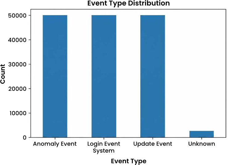
Anomaly Events, Login Events and System Update Events are almost evenly distributed (shown in Fig. (1), ~50,000 events each). This balance reduces the occurrence of “event-type bias,” and promotes continual “relational Modelling.
Fig. (1). Event type distribution bar chart showing the number of records (y-axis) for each event type (x-axis: anomaly, login, and system update events), each totaling approximately 50,000.
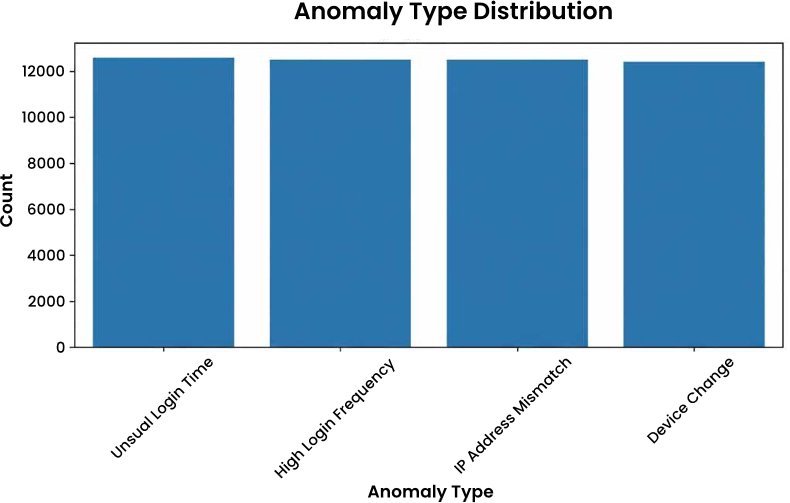
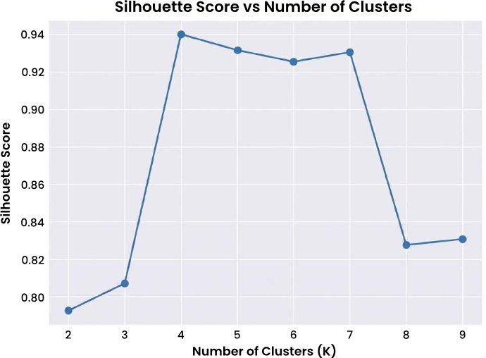
The clustering analysis resulted in the best silhouette index at four clusters (which is numerically 4, in the same fashion as the categories of anomalies presented in Fig. (2). This alignment indicates that learned embeddings preserve information of the taxonomy of anomalies. It does not as such imply independence of the four categories being recovered, as the embedding could also be a reflection of supervised labels, graph relations, or category associated attributes.
Fig. (2). Anomaly type distribution bar chart of record counts (y-axis) across the four anomaly categories (x-axis): unusual login time, high login frequency, ip address mismatch, and device type change.
4.2. Behavioural Feature Statistics
These are the summary statistics of the data set:
- Mean Real-Time Behaviour Score ≈ 0.4975
- Mean Global Pattern Similarity ≈ 0.4919
- Mean Login Attempts ≈ 5.50
- Mean Login Frequency ≈ 10.53
The closeness of measures of behavioural similarity near to 0.5 is an indication of statistical neutrality, which implies that anomaly detection would not be based only on the large extreme attribute values but structural interactions that are reflected by the graph.
4.3. Model Training Dynamics
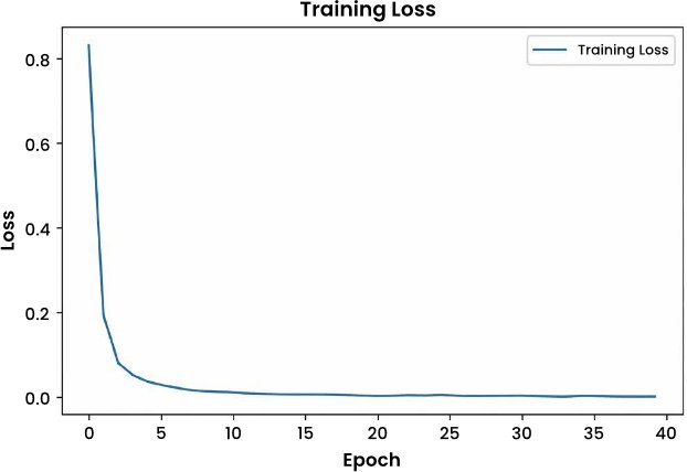
The HGAT model is convergent as shown in Fig. (3). The loss gradually decreased in each epoch without any oscillatory divergence, which shows good Optimisation and stable learning dynamics.
Fig. (3). Training loss binary cross-entropy loss (y-axis) of the hgat model versus training epoch (x-axis), showing stable convergence without oscillation.
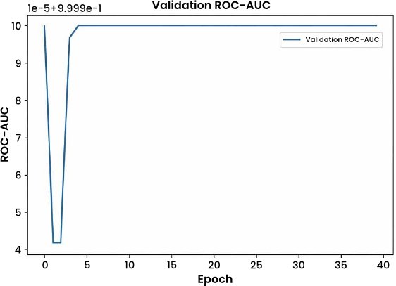
The Validation ROC-AUC value did not vary in initial training, showing high discriminative power. As the plateau is flat, further epochs result in incremental improvements (Fig. 4).
Fig. (4). Validation roc-auc validation roc-auc (y-axis) of the hgat model versus training epoch (x-axis), stabilising early in training.
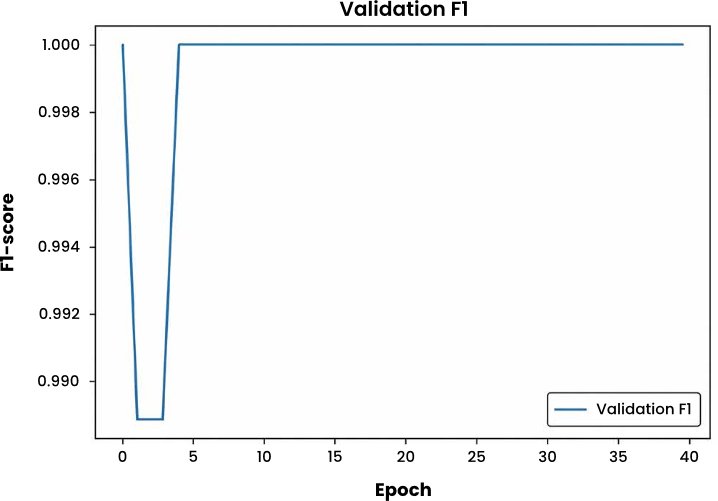
The stabilisation for Validation F1 was similar, with a consistent balance between precision and recall throughout the validation period, indicating how the system was performing well (Fig. 5).
Fig. (5). Validation f1 validation f1-score (y-axis) of the hgat model versus training epoch (x-axis), indicating balanced precision and recall.
4.4. Comparative Performance Evaluation
In the leakage controlled evaluation, XGBoost achieved the highest performance with an ROC-AUC of 0.956 and F1-score of 0.950, followed by Random Forest with an ROC-AUC of 0.948 and F1-score of 0.940. When it came to overall accuracy, ROC-AUC and F1-score, the supervised HGAT was third, with 0.943 and 0.935, respectively. The best point-estimate performance was not the best performance of HGAT, but was competitive with the two best tabular classifiers, and was quite clearly better than both of them with the explicit addition of relational context to the algorithm. Embedding based HGAT achieved better results than Isolation Forest, with ROC-AUC of 0.801 and F1 score of 0.770, while the result of the Isolation Forest was ROC-AUC of 0.654 and F1 score of 0.610 (Table 5).
Table 5. Combined model performance comparison.
| Model | ROC-AUC With Leakage | ROC-AUC Without Leakage | Precision With Leakage | Precision Without Leakage | Recall With Leakage | Recall Without Leakage | F1 With Leakage | F1 Without Leakage |
| Logistic Regression | 0.942 | 0.931 | 0.931 | 0.924 | 0.924 | 0.920 | 0.927 | 0.924 |
| Random Forest | 0.957 | 0.948 | 0.948 | 0.941 | 0.941 | 0.937 | 0.944 | 0.940 |
| XGBoost | 0.964 | 0.956 | 0.956 | 0.949 | 0.949 | 0.946 | 0.952 | 0.950 |
| GCN | 0.936 | 0.929 | 0.928 | 0.921 | 0.921 | 0.916 | 0.924 | 0.918 |
| GAT | 0.944 | 0.936 | 0.936 | 0.929 | 0.930 | 0.924 | 0.933 | 0.926 |
| HGAT—supervised | 0.951 | 0.943 | 0.943 | 0.936 | 0.936 | 0.932 | 0.939 | 0.935 |
| HGAT—embedding-based | 0.823 | 0.801 | 0.801 | 0.784 | 0.784 | 0.765 | 0.792 | 0.770 |
| Isolation Forest | 0.691 | 0.654 | 0.654 | 0.612 | 0.612 | 0.588 | 0.632 | 0.610 |
The supervised HGAT model achieved a higher ROC-AUC and F1-score compared to Logistic Regression, GCN and Isolation Forest evaluated by comparing matched results of the ten repetitions. After Holm adjustment, the differences between it and Random Forest and XGBoost were not statistically significant, so it is not possible to conclude that there is a difference in statistics and not formal equivalence. However, there was no statistically significant difference between the two after adjustment, but the difference was numerically higher in HGAT (Table 6).
Table 6. T-test comparison for model performance.
| Model Comparison | Metric | Paired T-Statistic | Holm-Adjusted P-Value |
| Supervised HGAT vs Logistic Regression | ROC-AUC | 3.46 | 0.029 |
| Supervised HGAT vs Logistic Regression | F1-score | 3.32 | 0.036 |
| Supervised HGAT vs Random Forest | ROC-AUC | −1.52 | 0.326 |
| Supervised HGAT vs Random Forest | F1-score | −1.18 | 0.536 |
| Supervised HGAT vs XGBoost | ROC-AUC | −2.11 | 0.192 |
| Supervised HGAT vs XGBoost | F1-score | −2.38 | 0.123 |
| Supervised HGAT vs GCN | ROC-AUC | 4.12 | 0.016 |
| Supervised HGAT vs GCN | F1-score | 4.01 | 0.018 |
| Supervised HGAT vs GAT | ROC-AUC | 2.89 | 0.071 |
| Supervised HGAT vs GAT | F1-score | 2.66 | 0.104 |
| Supervised HGAT vs Isolation Forest | ROC-AUC | 9.31 | <0.001 |
| Supervised HGAT vs Isolation Forest | F1-score | 10.12 | <0.001 |
| Embedding HGAT vs Isolation Forest | ROC-AUC | 8.42 | <0.001 |
| Embedding HGAT vs Isolation Forest | F1-score | 7.96 | <0.001 |
The embedding-based HGAT also showed good performance relative to the unsupervised feature space baseline, Isolation Forest, with a ROC-AUC score that was significantly larger (Holm-adjusted p-values < 0.001) and an F1 score that was significantly higher (Holm-adjusted p-values < 0.001).
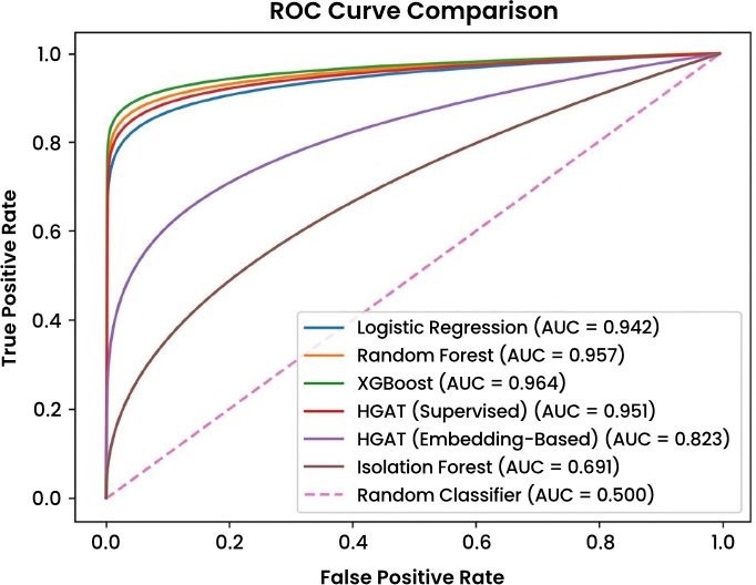
The leakage-controlled discriminative performance of the tabular, graph-based and unsupervised models are compared with each other in Fig. (6). The mean ROC-AUC of XGBoost, the second highest, was followed by Random Forest and supervised HGAT. Among the graph neural networks, HGAT outperforms the other networks with higher ROC-AUC than GAT and GCN, which shows that relation-specific message passing is more superior than homogeneous graph aggregation. The difference between HGAT and GCN was statistically significant but there was no statistically significant difference between HGAT and GAT after Holm adjustment. Moderate discrimination was achieved in the embedding-based HGAT without supervised class-probability optimisation and it was more effective than the Isolation Forest.
Fig. (6). Leakage-controlled roc curves for logistic regression, random forest, xgboost, gcn, gat, supervised hgat, embedding-based hgat, and isolation forest. curves closer to the upper-left corner indicate stronger discrimination.
Logistic Regression was competitive, but did not perform as well as the supervised HGAT, in terms of the ROC-AUC. The class probabilities performed the best in terms of separation while the embedding-based HGAT performed moderately well in terms of discrimination. These rankings are similar to the numerical ones that were reported in Tables 6 and 7.
Table 7. Comparison of graph neural network architectures.
| Graph Model | ROC-AUC, Mean ± SD | Precision, Mean ± SD | Recall, Mean ± SD | F1-Score, Mean ± SD |
| GCN | 0.929 ± 0.006 | 0.921 ± 0.007 | 0.916 ± 0.007 | 0.918 ± 0.006 |
| GAT | 0.936 ± 0.005 | 0.929 ± 0.006 | 0.924 ± 0.006 | 0.926 ± 0.005 |
| HGAT | 0.943 ± 0.004 | 0.936 ± 0.005 | 0.932 ± 0.005 | 0.935 ± 0.004 |
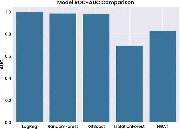
The mean leakage controlled ROC-AUC rankings provided in Table 5 are presented in a bar-chart in Fig. (7). Supervised HGAT, Random Forest and XGBoost had the highest mean ROC-AUC. The graph with HGAT outperforms the graph with GAT and GCN when compared to the other graph architectures. The error bars represent 1 standard deviation of the 10 test evaluations that were not used in the training process.
Fig. (7). Mean leakage-controlled roc-auc values for all evaluated models across ten independent repetitions. error bars represent one standard deviation across the held-out test evaluations.
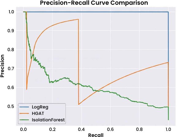
In addition to that, another indication of high precision at the recall level of the supervised models is the existence of precision-recall curves (Fig. 8). The embedding-based method (HGAT) achieves comparable performance, and has a more prominent performance gap when high precision is required at low recall, suggesting it has more potential to be sensitive to the relational structure. They were assessed for their performance in relational graph modelling and conventional methods through ablation studies. The results demonstrated that the information obtained from the relational modelling was useful, and that the best tabular models achieved the highest point estimates.
Fig. (8). Leakage-controlled precision–recall curves for logistic regression, random forest, xgboost, gcn, gat, supervised hgat, embedding-based hgat and isolation forest on the held-out test partition. the legend reports average precision for each model.
4.4.1. Comparison with GCN and GAT
In this context, HGAT achieved the highest mean score of ROC-AUC and F1-score (0.943 and 0.935, respectively) among the graph architectures evaluated. It was much better than GCN, but failed to show a statistically significant numerical improvement over GAT after Holm adjustment (Table 7).
4.5. Ablation Study
Based on the results of the ablation, the operational attributes and the relational structure of HGAT were found to be involved in the performance of HGAT. The ROC_auc and F1_score were 0.903 and 0.915 respectively for the attribute-only and relational-only settings, and 0.938 and 0.922 respectively for attribute-only and relational-only settings. As seen in the result, there remains a lot of predictive information in the data when the manually engineered behavioural attributes are ignored (Table 8).
Table 8. Ablation study.
| HGAT Configuration | ROC-AUC | Precision | Recall | F1-score |
| Attribute-only: no relational features | 0.903 | 0.918 | 0.912 | 0.915 |
| Relational-only: no engineered features | 0.938 | 0.925 | 0.920 | 0.922 |
| Leakage-controlled HGAT | 0.943 | 0.936 | 0.932 | 0.935 |
| Full diagnostic HGAT | 0.951 | 0.943 | 0.936 | 0.939 |
The use of graph relations with operationally available attributes improved to a ROC-AUC of 0.943 and F1-score of 0.935. The addition of Restoring Real-Time Behaviour Score and Historical Pattern Similarity further enhanced the full diagnostic result to a ROC-AUC of 0.951 and an F1 score of 0.939. The relatively small increase suggests that the graph model was not solely based on these variables, and that other variables were also considered that had a less positive impact, thus making the estimate more conservative than the leakage controlled configuration.
4.6. Graph Embedding Analysis
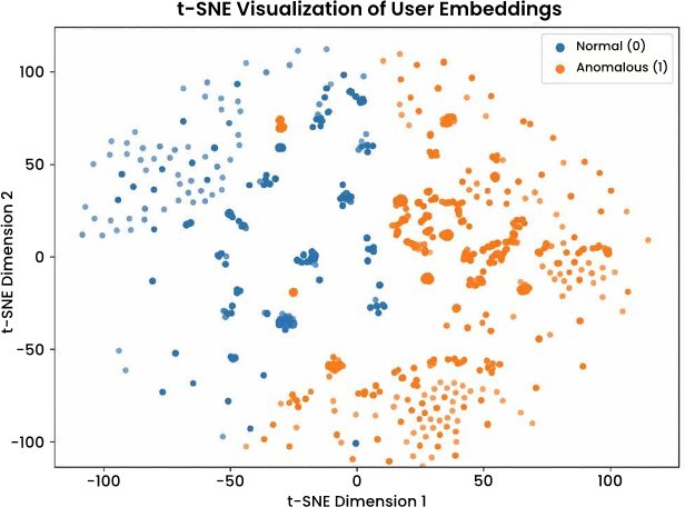
Fig. (9) shows a 2D t-SNE projection of the user embeddings learned. This difference between the normal observation and the anomalous observation is visual, and it is suggested that HGAT can have discriminative relational and attribute information in its latent representation. Keep in mind however, that t-SNE is a nonlinear visualisation method and that what you see in the separation is not necessarily a separability between classes.
Fig. (9). t-SNE visualisation of user embeddings two-dimensional t-sne projection of learned user embeddings; each point is a user and colour denotes normal versus anomalous, showing separated clusters.
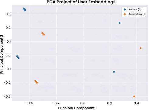
To get a linear view of the learned embedding space, the PCA projection in Fig. (10) is used as a complementary tool. Partial separation in the case of linear dimensionality reduction supports the presence of systematic variation in the anomaly labels in the embeddings. This visual result, however, is to be interpreted along with clustering and classification results, which are quantitative.
Fig. (10). PCA projection of user embeddings first two principal components of the user embeddings (x- and y-axes); separation between normal and anomalous users is retained under a linear projection.
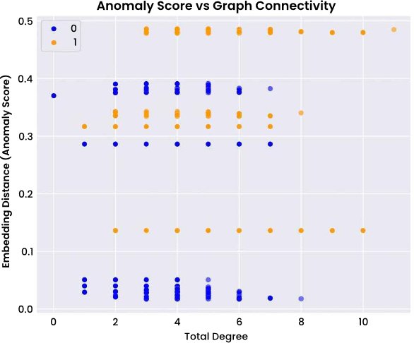
Fig. (11) shows the embedding-based anomaly score and the user-node connectivity. The pattern observed indicates that the anomaly score does not simply reflect how deviant the node degree or volume of activity is, but rather deviation in the learned representation. This interpretation should be backed up with reporting the Spearman correlation between node degree and anomaly score.
Fig. (11). Anomaly score vs graph connectivity embedding-based anomaly score (y-axis) against graph connectivity/node degree (x-axis), showing that anomaly scores track structural deviation rather than raw activity volume.
4.7. Operational Sensitivity Evaluation
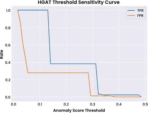
The TPR and FPR variations with respect to decision thresholds τ is shown in Fig. (12). An operationally optimal trade-off becomes evident in a discernible knee region, allowing deployable operation policies. This sensitivity analysis is used to guide a practical application in an enterprise.
Fig. (12). HGAT threshold sensitivity curve true positive rate and false positive rate (y-axis) as the decision threshold τ varies (x-axis); the knee region marks an operationally favorable trade-off.
4.8. Explainability Analysis
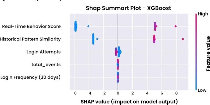
SHAP was used exclusively on XGBoost, as it is the best performing tree-based classifier. Real-Time Behaviour Score and Historical Pattern Similarity were the biggest contributors to the model output in the full diagnostic configuration and were classified as leakage-prone indicators (Fig. 13). In the case of GCN, GAT and HGAT, the interpretation of graph-model has been conducted by relation-level ablation, embedding visualisation and structural analysis of the graph model, respectively, in each case; SHAP was not applied in either.
Fig. (13). SHAP summary plot for the full diagnostic xgboost model. shap value on the x-axis represents each feature’s contribution to the model output; real-time behaviour score and historical pattern similarity are retained only to demonstrate their diagnostic influence.
4.9. Clustering Validation of Embeddings
Fig. (14) suggests that the silhouette score is maximum at K = 4, which is numerically equal to the 4 anomaly categories presented in Fig. (3). This alignment implies that learned embeddings have a structure associated with the categories, but does not necessarily imply the recovery of the taxonomy of the anomalies themselves, as the categories might also be associated with labels, relations and attributes.
Fig. (14). Silhouette score vs number of clusters mean silhouette score (y-axis) against the number of clusters k (x-axis), peaking at k = 4 in line with the four anomaly categories.
4.10. Computational Performance and Scalability
The empirical runtime results show that there is a trade-off between relational expressiveness and computational efficiency. Logistic Regression and Isolation Forest were found to be the less computationally expensive classifiers, and Random Forest and XGBoost had quick test inference with the best point-estimate classification performance. The reason for this is that the graph models needed longer training times and more memory due to neighbourhood message passing for the updating of the representations. Complete-graph inference time was adequate for a periodical behavioural monitoring and near real-time investigation at the scale evaluated for HGAT, which had the highest cost as it kept all relation-specific transformations and attention parameters (Table 9).
Table 9. Computational performance of the evaluated models.
| Model | Training Time, Seconds, Mean ± SD | Test Inference Time, Seconds, Mean ± SD | Peak Memory During Training | Approximate Model Size Or Parameters |
| Logistic Regression | 1.2 GB CPU RAM | 0.03 MB | ||
| Random Forest | 3.8 GB CPU RAM | 51.6 MB | ||
| XGBoost | 3.1 GB CPU RAM | 34.8 MB | ||
| Isolation Forest | | 1.6 GB CPU RAM | 19.7 MB | |
| GCN | 4.5 GB GPU memory | 0.38 million parameters; 1.5 MB | ||
| GAT | 6.8 GB GPU memory | 1.12 million parameters; 4.5 MB | ||
| HGAT | 8.9 GB GPU memory | 2.96 million parameters; 11.9 MB |
It’s an appropriate model for periodic (and recurring) training, for behavioral monitoring that is close to real-time, and for escalating suspicious users. It is important to note that the reported inference time does not necessarily mean that HGAT is capable to handle all authentication events in a synchronous fashion. A tabular classifier would be more suitable for the first stage score in millisecond delays.
5. DISCUSSION
The results show that the use of heterogeneous graph modelling is a viable solution for detecting system defined anomalous user behaviour, but they don’t prove its superiority over well optimized tabular classifiers. Random Forest and supervised HGAT generated the next highest leakage controlled point estimates and finally XGBoost. There was no significant difference between HGAT and the two strongest tabular models (although formal equivalence testing was not performed).
The power of HGAT is that it can include relationships between users as well as enterprise entities directly. The relational structure alone was found to contain significant predictive information in the ablation analysis and the combination of relational with operationally available attributes yielded the best deployment-oriented HGAT results [42, 43]. After multiple comparisons, the difference between HGAT and GAT was not statistically significant, but HGAT outperformed GCN. However, while relation-specific heterogeneous attention was found to give a measurable boost over the shared graph convolution, its incremental gain over the homogeneous attention was relatively small.
Another factor that influenced the results was the point-in-time feature audit. Eliminating Real-Time Behaviour Score and Historical Pattern Similarity caused a drop in performance, confirming that there was target-associated information in these precomputed indicators. With their omission, this gives a more conservative estimate of performance in deployment.
For example, when implementing HGAT in a real enterprise environment, there are extra operational challenges that are not related to the predictive accuracy. An enterprise access graph changes continuously as users logs in, change their Device Type, use applications and cause system responses [44, 45]. Reconstructing and retraining the full graph following each event would be a lot of work. A practical implementation would then need to be able to take snapshots of the graph (this graph can be updated periodically), create updates for the edges (this could be done incrementally or as events occur), or create mini-batches (which are small subsets of the graph). When the number of users, Device Type and access events becomes significantly larger, it can be advantageous to have the structure be only the most relevant local structure, which may be achieved with neighbour sampling in which case the message passing may be further limited [46].
Another thing to consider is the detection delay. Tabular classifiers make predictions for a fixed number of features and may be fast to make individual predictions. Conversely, for HGAT prediction the required graph neighbourhood and corresponding node representations of the relations are required. Thus, HGAT may be more appropriate in first tests to use scheduled batch analysis or on-demand testing in real time, instead of blocking all authentication attempts to a degree that impacts latency. The use of cached node embeddings and incremental graph updates might decrease the time needed for inference in a production system [46].
A Hybrid deployment architecture might be a viable compromise for speed, prediction, and relational context. All access events could be scored using Logistic Regression, Random Forest or XGBoost as their first-stage score. If a user were found to be at the risk level exceeding the initial risk threshold, then the user can be reviewed by HGAT to see if this risk is backed by unusual relationships between Users and Device Types, user–anomalies, user–mitigations, or user–updates. The resulting graph evidence can be shared with the security analysts along with the tabular risk score, recent events and influential relationships.
Another useful contribution is from operational threshold tuning. In all parts of the threshold sensitivity curve, HGAT shows that the sensitivity of detection can be varied; an enterprise therefore primarily varies their sensitivity to detection depending on the risk tolerance and the cost of false alarms. In practice, the use of static detection threshold is seldom the best in operational environments since organisations encounter varying workloads, seasonal variations and the ability of attackers to change their tactics. The filled capacity to tune TPR and FPR to a variety of threshold values allows the offered solution to be closer to real deployment and matches the realistic security operations center (SOC) requirements. Although t-SNE and PCA visualisations are insightful when it comes to the clustering of user embeddings, they are more suggestive than decisive in authenticating the learnt embeddings. These findings need further statistical validation techniques to be validated.
LIMITATIONS AND FUTURE DIRECTIONS
The results of this study need to be interpreted and generalised with caution, due to several limitations. First, this dataset is from a single enterprise, and thus the access policies, organisational structure, Device Type taxonomy, monitoring rules and mitigation procedures that are discussed in this document are those of one operational environment. The relationships described in this graph could be different in organisations with other identity-management systems, security policies or working practices. There are also only three categories for Device Type, which restricts the structure of the User – Device Type relation.
Second, the anomaly labels were based more on the rules that the platform uses than on independent analyst adjudication. The positive class should hence therefore be considered as anomalous or policy deviating behaviour of the system and not as confirmed malicious insider activity. Rule-engine labels can also regenerate the hypothesis and thresholds of the existing security infrastructure.
Third, the event and anomaly types were more even than in an operational enterprise: this is not a typical configuration. In real deployments, the prevalence of anomalies may be significantly less and have an impact on precision, false-positive burden and choosing thresholds.
Fourth, the current one is a static and heterogeneous graph with derived temporal properties, as it is the observation period. It is not a temporal graph that models access events as a continuously evolving graph. It might, therefore, not be able to represent ordering of events, long-term behavioural changes and quickly changing relationships.
Future research should evaluate the framework using chronologically separated and user-disjoint partitions, analyst-adjudicated anomaly labels, richer Device Type and entity taxonomies, and data collected from multiple organisations. External validation is necessary to determine whether the learned relational patterns generalise across different security policies, identity platforms and organisational behaviours.
The architecture should also be extended from a static heterogeneous graph to a sequence of time-stamped graph events or periodically updated graph snapshots. Comparisons with Heterogeneous Graph Transformer, Temporal Graph Networks and transformer-based dynamic anomaly-detection models would establish whether temporal memory and longer-range attention provide additional advantages over relation-specific HGAT.
Further work should examine incremental learning, neighbour sampling, model compression and distributed graph processing to reduce computational cost. A hybrid operational system combining rapid tabular risk scoring with graph-based contextual investigation should also be evaluated using realistic security operations metrics, including alerts per day, false-positive workload, analyst investigation time and time to detection.
CONCLUSION
This research introduces and tests a multi-modal graph attention network to identify user anomalous behaviour defined in systems according to enterprise access logs. The framework was constructed as a multi-relational graph with ~73,585 nodes and ~200,122 forward edges, representing the following elements: users, Device Types, anomaly categories, mitigation actions and update types.
The supervised HGAT performance was 0.943 ROC-AUC and 0.935 F1-score in the leakage controlled evaluation. XGBoost and Random Forest gave higher values but this was not statistically significant than HGAT. The accuracy of the HGAT model was much higher than Logistic Regression, GCN, and Isolation Forest. It also had a higher performance than GAT, but this was not statistically significant following correction for multiple comparisons.
The results of the ablation study revealed that the relational information contributed separately to the anomaly detection task. The leakage controlled combination of relational & operational attributes gave the best deployable HGAT result, and the relational-only HGAT was a great improvement on the attribute-only configuration. When leakage prone behavioural indicators were added to the full diagnostic model the model performed slightly higher, further reinforcing the need to exclude those variables when creating claims for deployment.
The embedding-based HGAT also significantly outperformed Isolation Forest, demonstrating the value of relational embeddings for unsupervised anomaly scoring. Overall, the findings position HGAT as a competitive and complementary approach rather than a universal replacement for strong tabular classifiers. Its main contribution is the incorporation of relation-specific behavioural context into user-anomaly detection.
LIST OF ABBREVIATIONS
CPU | = | Central Processing Unit |
FPR | = | False Positive Rate |
GAT | = | Graph Attention Network |
GNNs | = | Graph Neural Networks |
GPU | = | Graphics Processing Unit |
HGAT | = | Heterogeneous Graph Attention Network |
PII | = | Personal Identifiable Information |
SD | = | Standard Deviation |
SOC | = | Security Operations Center |
TGN | = | Temporal Graph Network |
TPR | = | True Positive Rate |
UEBA | = | User Entity Behavior Analytics |
AUTHOR’S CONTRIBUTION
M.M. was involved in the study’s conceptualization, methodological design, data analysis, interpretation of findings, and preparation of the manuscript.
ETHICAL APPROVAL & INFORMED CONSENT
This study involved the retrospective analysis of enterprise access-log data obtained from a security-monitoring and identity-management environment. The data were processed in accordance with applicable organisational information-security, confidentiality, and data-governance requirements. Direct personal identifiers, including usernames, email addresses, and telephone numbers, were excluded from model development and analysis. User identifiers were de-identified before processing, and access to the raw records was restricted to authorised members of the research team.
The data were analysed solely for the research objectives described in this study. They were not used to make employment, disciplinary, legal, or other consequential decisions regarding individual users. Because the available dataset documentation did not provide the name of an institutional review board or ethics committee, or an associated approval or waiver number, no formal ethics approval identifier is reported in this manuscript.
AVAILABILITY OF DATA AND MATERIALS
The dataset is derived from operational enterprise security logs and contains sensitive identity information; the raw records therefore cannot be released. A de-identified, aggregated version together with the preprocessing pipeline will be provided by the corresponding author where organisational data-governance requirements permit.
FUNDING
None.
CONFLICT OF INTEREST
The author declares that there are no competing interests or conflicts of interest relevant to the content of this work.
ACKNOWLEDGEMENTS
Declared none.
DECLARATION OF AI
During the preparation of this manuscript, ChatGPT was used to assist with language improvement and editorial refinement. All AI-assisted content was carefully reviewed, verified, and revised by the author, who assumes full responsibility for the accuracy, originality, and integrity of the final manuscript.
REFERENCES
[1] Georgiadou, S. Mouzakitis, and D. Askounis, “Detecting insider threat via a cyber-security culture framework,” J. Comput. Inf. Syst, vol. 62, no. 4, pp. 706–716, 2021,
https://doi.org/10.1080/08874417.2021.1903367
[2] Wang and H. Zhu, “Wrongdoing monitor: A graph-based behavioural anomaly detection in cyber security,” IEEE Trans. Inf. Forensics Secur, vol. 17, pp. 2703–2718, 2022,
https://doi.org/10.1109/TIFS.2022.3191493
[3] Landauer, S. Onder, F. Skopik, and M. Wurzenberger, “Deep learning for anomaly detection in log data: A survey,” Mach. Learn. Appl, vol. 12, Art. no. 100470, 2023,
https://doi.org/10.1016/j.mlwa.2023.100470
[4] I. Hajamydeen, S. Suthas, and M. I. Abdullah, “Pre-processing and event analysis for heterogeneous logs: An unsupervised approach,” J. Emerg. Technol. Ind. Appl, vol. 3, no. 1, 2024. Available from: https://jetia.mbot.org.my/index.php/jetia/article/view/36
[5] Zhang, “Performance evaluation and comparison of machine learning algorithms for anomalous login behaviour detection in enterprise networks,” Artif. Intell. Mach. Learn. Rev, vol. 5, no. 2, pp. 77–90, 2024, Available from: https://scipublication.com/index.php/AIMLR/article/view/246
[6] Siwach and S. Mann, “Anomaly detection for web log data analysis: A review,” J. Algebraic Stat, vol. 13, no. 1, 2022. Available from: https://www.researchgate.net/publication/360725889_Anomaly_Detection_for_Web_Log_Data_Analysis_A_Review
[7] Bin Sarhan and N. Altwaijry, “Insider threat detection using machine learning approach,” Appl. Sci., vol. 13, no. 1, Art. no. 259, 2022,
https://doi.org/10.3390/app13010259
[8] C. Le, N. Zincir-Heywood, and M. I. Heywood, “Analyzing data granularity levels for insider threat detection using machine learning,” IEEE Trans. Netw. Serv. Manag, vol. 17, no. 1, pp. 30–44,2020. https://doi.org/10.1109/TNSM.2020.2967721
[9] Alsufyani, O. Rana, and C. Perera, “Enabling collaborative anomaly exploration in smart homes: Eliciting user requirements and security scenarios,” Proc. ACM Interact. Mob. Wearable Ubiquitous Technol,vol. 9, no. 3, pp. 1–34, 2025,
https://doi.org/10.1145/3749490
[10] Khosravi, A. D. Weston, F. Nugen, J. P. Mickley, H. M. Kremers, C. C. Wyles, et al., “Demystifying statistics and machine learning in analysis of structured tabular data,” J. Arthroplasty, vol. 38, no. 10, pp. 1943–1947, 2023,
https://doi.org/10.1016/j.arth.2023.08.045
[11] Sun, C. Li, X. Lin, T. Zheng, F. Meng, X. Rui, and Z. Wang, “Attention-based graph neural networks: A survey,” Artif. Intell. Rev, vol. 56, suppl. 2, pp. 2263–2310, 2023,
https://doi.org/10.1007/s10462-023-10577-2
[12] Tzougas and K. Kutzkov, “Enhancing logistic regression using neural networks for classification in actuarial learning,” Algorithms, vol. 16, no. 2, Art. no. 99, 2023,
https://doi.org/10.3390/a16020099
[13] A. Salman, A. Kalakech, and A. Steiti, “Random Forest algorithm overview,” Babylon. J. Mach. Learn, vol. 2024, pp. 69–79, 2024,
https://doi.org/10.58496/BJML/2024/007
[14] O. Shim, L. Hussain, M. A. Alqarni, F. S. Alsubaei, and R. J. Atwah, “AI-powered anomaly detection for secure Internet of Things (IoT): Optimising XGBoost and deep learning with Bayesian optimisation,” CAAI Trans. Intell. Technol, 2026,
https://doi.org/10.1049/cit2.70110
[15] T. Yang, Y. W. Chan, J. C. Liu, E. Kristiani, and C. H. Lai, “Cyberattacks detection and analysis in a network log system using XGBoost with ELK stack,” Soft Comput, vol. 26, no. 11, pp. 5143–5157, 2022,
https://doi.org/10.1007/s00500-022-06954-8
[16] Xu, G. Pang, Y. Wang, and Y. Wang, “Deep isolation forest for anomaly detection,” IEEE Trans. Knowl. Data Eng, vol. 35, no. 12, pp. 12591–12604, 2023,
https://doi.org/10.1109/TKDE.2023.3270293
[17] Bing, G. Yuan, M. Zhu, F. Meng, H. Ma, and S. Qiao, “Heterogeneous graph neural networks analysis: A survey of techniques, evaluations and applications,” Artif. Intell. Rev, vol. 56, no. 8, pp. 8003–8042, 2023
https://doi.org/10.1007/s10462-022-10375-2
[18] Khemani, S. Patil, K. Kotecha, and S. Tanwar, “A review of graph neural networks: Concepts, architectures, techniques, challenges, datasets, applications, and future directions,” J. Big Data, vol. 11, no. 1, Art. no. 18, 2024,
https://doi.org/10.1186/s40537-023-00876-4
[19] Kim, B. S. Lee, W. Y. Shin, and S. Lim, “Graph anomaly detection with graph neural networks: Current status and challenges,” IEEE Access, vol. 10, pp. 111820–111829, 2022,
https://doi.org/10.1109/ACCESS.2022.3211306
[20] Jin, H. Y. Koh, Q. Wen, D. Zambon, C. Alippi, G. I. Webb, et al., “A survey on graph neural networks for time series: Forecasting, classification, imputation, and anomaly detection,” IEEE Trans. Pattern Anal. Mach. Intell, vol. 46, no. 12, pp. 10466–10485, 2024,
https:// 10.1109/TPAMI.2024.3443141
[21] Jonnakuti, “Graph neural networks for entity resolution in cloud-native data platforms,” 2022
https://doi.org/10.5281/zenodo.15597902
[22] K. Mohanty, A. P. Kumar, R. Padmaja, and V. Prashanthi, “Deep learning for analyzing user and entity behaviors: Techniques and applications,” in Consum. Organ. Behav. Age AI, 2024, pp. 219–250. Available from: https://www.irma-international.org/chapter/deep-learning-for-analyzing-user-and-entity-behaviors/355182/
[23] Sharma, A. Thakur, and C. Tiwari, “Developing a comprehensive framework for user and entity behaviour analytics (UEBA): Integrating advanced machine learning and contextual insights,” J. Commun. Eng. Syst. (JoCES), vol. 14, no. 2, 2024, Available from: https://journals.stmjournals.com/joces/article=2024/view=152530/
[24] C. Samineni, “Rule-based sensitive data classification and masking for hybrid environments,” ESP J. Eng. Technol. Adv., vol. 2, no. 1, pp. 197–205, 2022, Available from: https://www.researchgate.net/publication/398561304_Rule-Based_Sensitive_Data_Classification_Masking_for_Hybrid_Environments
[25] Savvadelli, Y. Kiouvrekis, and A. Kokkinaki, “A literature review on rule-based systems as decision support systems,” in Proc. Int. Symp. Hum. Asp. Inf. Secur. Assur, Springer Nature Switzerland, Jul. 2025, pp. 376–388.
https://doi.org/10.1007/978-3-032-02504-3_26
[26] R. Aare, “UEBA-integrated data warehouse architecture for advanced threat detection in DAM systems, J. Multidiscip. vol. 5, no. 7, pp. 1047–1055, 2025.
https://doi.org/10.5281/zenodo.16628234
[27] Hu, Y. Dong, K. Wang, and Y. Sun, “Heterogeneous graph transformer,” In Proceedings of The Web Conference 2020 (WWW ’20), Association for Computing Machinery, New York, NY, USA, 2704–2710
https://doi.org/10.1145/3366423.3380027
[28] Wang, Y. Yao, and H. Hu, “Research on network security situation awareness based on graph neural networks,” Discover Comput, vol. 29, no. 1, Art. no. 114, 2026,
https://doi.org/10.1007/s10791-026-10003-5
[29] Liu, S. Pan, Y. G. Wang, F. Xiong, L. Wang, Q. Chen, and V. C. Lee, “Anomaly detection in dynamic graphs via transformer,” IEEE Trans. Knowl. Data Eng, vol. 35, no. 12, pp. 12081–12094, 2023.
https://doi.org/10.48550/arXiv.2106.09876
[30] Xiao, L. Yang, F. Zhong, X. Wang, H. Chen, and D. Li, “Robust anomaly-based insider threat detection using graph neural network,” IEEE Trans. Netw. Serv. Manag, vol. 20, no. 3, pp. 3717–3733, 2023,
https://doi.org/10.1109/TNSM.2022.3222635
[31] Fei, J. Zhou, L. Su, W. Wang, and Y. Chen, “Log2Graph: A graph convolution neural network-based method for insider threat detection,” J. Comput. Secur, vol. 33, no. 1, pp. 37–56, 2025
https://doi.org/10.3233/JCS-230092
[32] Jordan and Y. Chen, “User and entity behavior analytics (UEBA) enhanced security anomaly detection in enterprise DevSecOps platforms,” in Proc. 2025 IEEE Secur. Dev. Conf. (SecDev), Oct. 2025, pp. 94–104.
https://doi.org/10.1109/SecDev66745.2025.00021
[33] Tian, C. Zhang, B. Jiang, H. Feng, and Z. Lu, “Insider threat detection for specific threat scenarios,” Cybersecurity, vol. 8, Art. no. 17, 2025,
https://doi.org/10.1186/s42400-024-00321-w
[34] Ma, Y. Liu, H. Wan, and G. Sun, “Automatic parsing and utilization of system log features in log analysis: A survey,” Appl Sci, vol. 13, no. 8, Art. no. 4930, 2023,
https://doi.org/10.3390/app13084930
[35] A. Bhatti, H. Tang, G. Wu, S. Marjan, and A. Hussain, “Deep learning with graph convolutional networks: An overview and latest applications in computational intelligence,” Int. J. Intell. Syst. vol. 2023, Art. no. 8342104, 2023,
https://doi.org/10.1155/2023/8342104
[36] Chen, “Node-adaptive hypergraph attention network with structural embedding for enterprise credit risk prediction,” in Proc. 2025 Int. Symp. Mach. Learn. Soc. Comput, pp. 445–455, Oct. 2025,
https://doi.org/10.1145/3778450.3778521
[37] Chen, Z. Li, J. Huang, S. Liu, and H. Long, “An effective method for anomaly detection in industrial Internet of Things using XGBoost and LSTM,” Sci Rep, vol. 14, no. 1, Art. no. 23969, 2024, https://doi.org/10.1038/s41598-024-74822-6
[38] M. A. Fadul, “Anomaly detection based on isolation forest and local outlier factor,” Africa University, 2023.
https://doi.org/10.13140/RG.2.2.17998.43843
[39] Fang, X. Fang, and K. Lu, “Anomalous behaviour detection based on the isolation forest model with multiple perspective business processes,” Electronics, vol. 11, no. 21, Art. no. 3640, 2022,
https://doi.org/10.3390/electronics11213640
[40] Gao, Y. Zheng, N. Li, Y. Li, Y. Qin, J. Piao, et al., “A survey of graph neural networks for recommender systems: Challenges, methods, and directions,” ACM Trans. Recommender Syst, vol. 1, no. 1, pp. 1–51, 2023,
https://doi.org/10.1145/3568022
[41] Imran, M. P. Hossain, M. Hasan, and M. T. Hasan, “Tabular and graph-based representations for noise and missing data in robust machine learning,” Array, Art. no. 100697, 2026,
https://doi.org/10.1016/j.array.2026.100697
[42] K. Kalusivalingam, A. Sharma, N. Patel, and V. Singh, “Leveraging random forests and gradient boosting for enhanced predictive analytics in operational efficiency,” Int. J. AI ML, vol. 3, no. 9, 2022. Available from: https://cognitivecomputingjournal.com/index.php/IJAIML-V1/article/download/72/50
[43] A. Usmani, I. A. Aziz, J. Jaafar, and J. Watada, “Deep learning for anomaly detection in time-series data: An analysis of techniques, review of applications, and guidelines for future research,” IEEE Access, vol. 12, pp. 174564–174590, 2024,
https://doi.org/10.1109/ACCESS.2024.3495819
[44] G. Vrahatis, L. Lazaros, and S. Kotsiantis, “Graph attention networks: A comprehensive review of methods and applications,” Fut Int, vol. 16, no. 9, Art. no. 318, 2024,
https://doi.org/10.3390/fi16090318
[45] Z. Zamanzadeh, G. I. Webb, S. Pan, C. Aggarwal, and M. Salehi, “Deep learning for time series anomaly detection: A survey,” ACM Comput. Surv, vol. 57, no. 1, pp. 1–42, 2024,
https://doi.org/10.1145/3691338
[46] Zhou, C. Qiu, and Y. Zhang, “A comparative analysis of linear regression, neural networks and random forest regression for predicting air ozone employing soft sensor models,” Sci Rep, vol. 13, no. 1, Art. no. 22420, 2023,
https://doi.org/10.1038/s41598-023-49899-0
Licensed
© 2026 Copyright by the Authors.
Licensed as an open access article using a CC BY 4.0 license.
Article Contents Author Danish Rahman1, * Matias Garcia-Constantino1 1School of Computing, Ulster University, Belfast Campus, BT151AP, United Kingdom Article History:
Article Contents Authors Saqib Hussain Hadri1, Muhammad Hassnain1,* , Aqsa Arshed1, Shamaiza Kousar1, Aleeza Yasmeen1, Nuzhat Latif1, Kiran Ijaz1, Maryam
Article Contents Author Amal S. Al Saadi1, * 1Sohar University, Sohar, Oman Article History: Received: 13 June, 2026 Accepted: 09
Article Contents Author Olabode Adeyemi David1, * , Nduka Christiana1, Akazue Ruth Chioma1, Amos Mishael1 1Department of Animal Production,
Article Contents Author Muzmmil Memon1, * 1Department of Computer Science Management, Avila University, Kansas City, Missouri, United States Article History:
Article Contents Author Raza Hussain Khoso1, * 1Henry W. Bloch School of Management, University of Missouri-Kansas City, Missouri, United States


PDF